Please wait a minute...
E-mail Alert Rss
 
物探与化探  2023, Vol. 47 Issue (5): 1316-1325    DOI: 10.11720/wtyht.2023.1605
  方法研究·信息处理·仪器研制 本期目录 | 过刊浏览 | 高级检索 |
基于B样条插值的瞬变电磁响应一维精确计算
邢涛1(), 王垚2, 李建慧2,3()
1.北京探创资源科技有限公司,北京 100071
2.中国地质大学(武汉) 地球物理与空间信息学院,湖北 武汉 430074
3.中国地质大学(武汉) 地质过程与矿产资源国家重点实验室,湖北 武汉 430074
One-dimensional accurate calculation of transient electromagnetic responses based on B-spline interpolation
XING Tao1(), WANG Yao2, LI Jian-Hui2,3()
1. Beijing Tanchuang Resources Technology Co., Ltd., Beijing 100071, China
2. School of Geophysics and Geomatics, China University of Geosciences (Wuhan), Wuhan 430074, China
3. State Key Laboratory of Geological Processes and Mineral Resources, China University of Geosciences (Wuhan), Wuhan 430074, China
全文: PDF(4095 KB)   HTML
输出: BibTeX | EndNote (RIS)      
摘要 

基于频谱法的瞬变电磁法一维正演策略中,多个计算环节对瞬变电磁响应计算精度有重要影响。为了提高一维正演效率,通常只直接计算数十个频点的频率域电磁响应,再采用三次样条插值将频率域电磁响应扩展至数百个频点。尽管三次样条插值函数计算的数值结果已能满足大多数正演需求,但其计算精度仍有提升空间。本文将高次B样条插值引入至瞬变电磁法一维正演,用于代替传统三次样条插值,并以磁偶源和圆形回线源为例验证了方法准确性。结果表明,对于多个地电模型,基于高次B样条插值计算的瞬变电磁响应精度均优于基于传统三次样条的计算结果。

服务
把本文推荐给朋友
加入引用管理器
E-mail Alert
RSS
作者相关文章
邢涛
王垚
李建慧
关键词 瞬变电磁法一维正演B样条插值    
Abstract

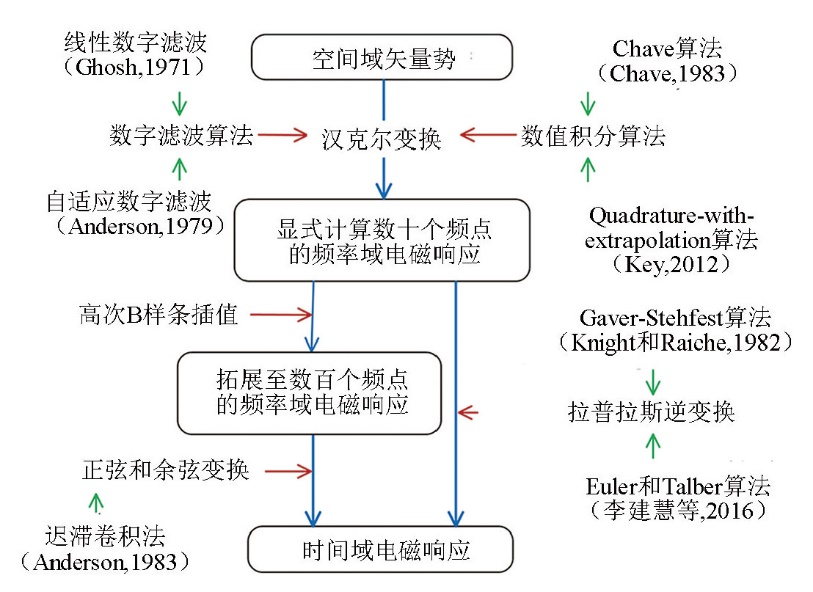
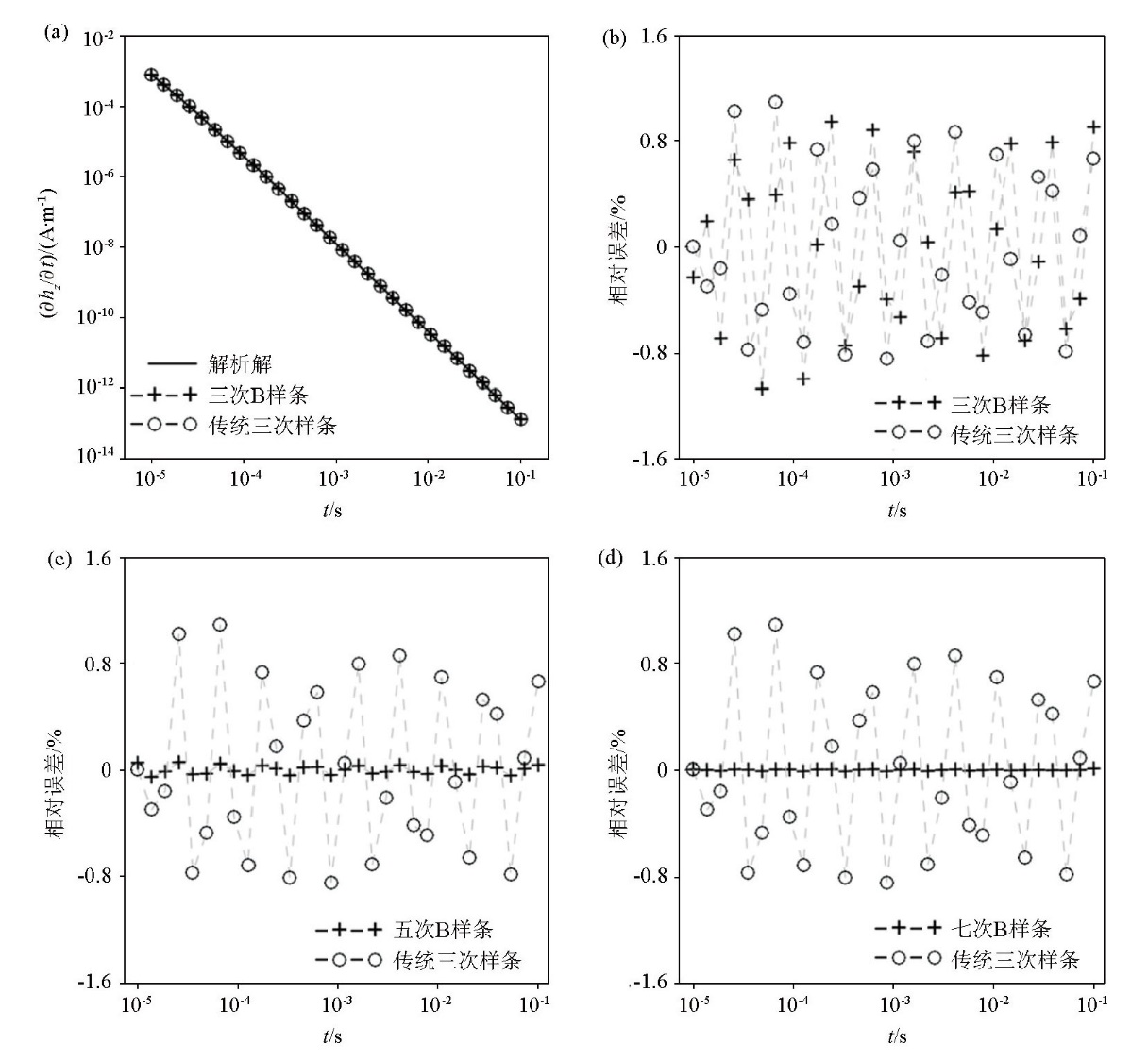
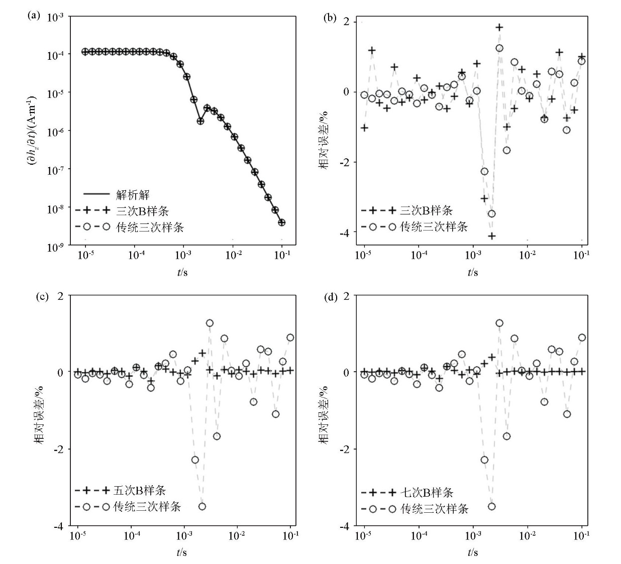
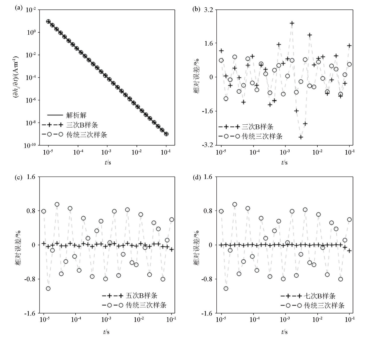
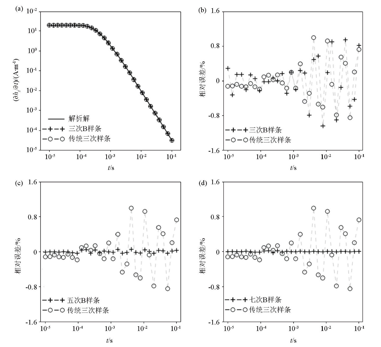
In the one-dimensional (1D) forward modeling of transient electromagnetic (TEM) responses based on spectral methods, multiple calculation steps significantly influence the calculation accuracy of TEM responses. To improve the efficiency of 1D forward modeling, the common practice is to directly calculate the frequency-domain electromagnetic responses of dozens of frequency points and then obtain the responses of hundreds of frequency points through cubic spline interpolation. Although the numerical results calculated using the cubic spline interpolation function can meet the requirements of most forward modeling scenarios, their accuracy can be further improved. This study introduced high-order B-spline interpolation into the 1D forward modeling of TEM responses to replace the conventional cubic spline interpolation and verified the accuracy of the method based on magnetic dipole sources and circle-shaped loop sources. The results show that the TEM responses of several geoelectric models calculated based on high-order B-spline interpolation exhibit higher accuracy than those calculated using conventional cubic spline interpolation.

Key wordstransient electromagnetics    one-dimensional forward modeling    B-spline interpolation
收稿日期: 2022-12-09      修回日期: 2023-04-18      出版日期: 2023-10-20
ZTFLH:  P631  
基金资助:国家自然科学基金(42022030)
通讯作者: 李建慧
作者简介: 邢涛(1983-),男,硕士,高级工程师,长期从事地球物理勘探方面的研究工作。Email:156663062@qq.com
引用本文:   
邢涛, 王垚, 李建慧. 基于B样条插值的瞬变电磁响应一维精确计算[J]. 物探与化探, 2023, 47(5): 1316-1325.
XING Tao, WANG Yao, LI Jian-Hui. One-dimensional accurate calculation of transient electromagnetic responses based on B-spline interpolation. Geophysical and Geochemical Exploration, 2023, 47(5): 1316-1325.
链接本文:  
https://www.wutanyuhuatan.com/CN/10.11720/wtyht.2023.1605      或      https://www.wutanyuhuatan.com/CN/Y2023/V47/I5/1316
Fig.1  瞬变电磁法一维正演技术路线
Fig.2  每数量级5个频点计算条件下垂直磁偶源位于1 000 Ω·m均匀半空间表面激发的磁场脉冲响应
a—三次B样条数值解;b—三次B样条相对误差曲线;c—五次B样条相对误差曲线;d—七次B样条相对误差曲线
插值算法 平均误差率/%
4频点 5频点 6频点 7频点 8频点 9频点
传统三次样条 9.08×10⁻¹ 5.27×10⁻¹ 3.75×10⁻¹ 2.60×10⁻¹ 3.21×10⁻¹ 2.19×10⁻¹
三次B样条 9.11×10⁻¹ 5.54×10⁻¹ 3.68×10⁻¹ 2.70×10⁻¹ 3.10×10⁻¹ 2.17×10⁻¹
四次B样条 7.20×10⁻¹ 4.02×10³ 1.50×10² 1.00×101 6.22×10⁻² 3.01×10⁻²
五次B样条 6.53×10⁻² 2.74×10⁻² 1.28×10⁻² 3.70×10⁻² 5.71 6.31×101
六次B样条 1.03×10³ 5.61×10⁻¹ 4.46×10⁻³ 2.03×10⁻³ 1.65×10⁻³ 1.29×10⁻³
七次B样条 1.53×10⁻² 4.22×10⁻³ 2.65×10² 1.15 3.47×10⁻⁴ 3.64×10⁻⁴
八次B样条 4.03×101 1.26 9.43×10⁻⁴ 2.16×10⁻² 1.08×10³ 1.53
九次B样条 4.13 1.81×10⁻³ 2.57×101 3.72×10⁻³ 2.52×10⁻⁴ 2.89×10⁻⁴
Table 1  垂直磁偶源位于1 000 Ω·m均匀半空间时不同插值算法产生的平均误差率
插值算法 最大相对误差/%
4频点 5频点 6频点 7频点 8频点 9频点
传统三次样条 1.81 1.09 7.24×10⁻¹ 4.57×10⁻¹ 6.98×10⁻¹ 8.82×10⁻¹
三次B样条 1.93 1.06 6.89×10⁻¹ 5.50×10⁻¹ 6.66×10⁻¹ 9.21×10⁻¹
四次B样条 1.38 2.60×10⁴ 1.59×10³ 1.12×10² 6.56×10⁻¹ 1.26×10⁻¹
五次B样条 1.31×10⁻¹ 5.60×10⁻² 2.50×10⁻² 1.01×10⁻¹ 2.17×101 5.25×10²
六次B样条 5.19×10³ 7.74 3.39×10⁻² 1.17×10⁻² 9.84×10⁻³ 6.47×10⁻³
七次B样条 9.31×10⁻² 1.08×10⁻² 2.36×10³ 1.35×101 1.62×10⁻³ 1.81×10⁻³
八次B样条 1.48×10² 1.82×101 1.47×10⁻² 5.29×10⁻² 9.53×10³ 1.36×101
九次B样条 4.77×101 8.67×10⁻³ 1.62×10² 4.68×10⁻² 5.12×10⁻³ 2.08×10⁻³
Table 2  垂直磁偶源位于1000 Ω·m均匀半空间时不同插值算法产生的最大相对误差
Fig.3  每数量级5个频点计算条件下垂直磁偶源位于1 Ω·m均匀半空间表面激发的磁场脉冲响应
a—三次B样条数值解;b—三次B样条相对误差曲线;c—五次B样条相对误差曲线;d—七次B样条相对误差曲线
插值算法 平均误差率/%
4频点 5频点 6频点 7频点 8频点 9频点
传统三次样条 1.71 5.59×10⁻¹ 3.11×10⁻¹ 1.82×10⁻¹ 5.64×10⁻² 5.69×10⁻²
三次B样条 1.21×101 7.83×10⁻¹ 3.16×10⁻¹ 1.49×10⁻¹ 7.80×10⁻² 5.66×10⁻²
四次B样条 4.76×10⁻¹ 8.95 7.80×10⁻¹ 1.03×10⁻¹ 2.40×10⁻² 1.42×10⁻²
五次B样条 1.02 7.57×10⁻² 3.21×10⁻² 1.46×10⁻² 1.07×10⁻² 4.93×10⁻²
六次B样条 4.31×101 1.08 3.12×10⁻² 5.84×10⁻³ 1.36×10⁻³ 9.76×10⁻⁴
七次B样条 1.55 5.09×10⁻² 1.33 2.11×10⁻² 8.84×10⁻⁴ 3.44×10⁻⁴
八次B样条 3.54 8.14×10⁻¹ 1.09×10⁻² 1.00×10⁻³ 6.33×10⁻² 4.56×10⁻⁴
九次B样条 8.00 3.74×10⁻² 2.78×10⁻¹ 1.13×10⁻³ 2.54×10⁻⁴ 4.82×10⁻⁵
Table 3  垂直磁偶源位于1 Ω·m均匀半空间时不同插值算法产生的平均误差率
插值算法 最大相对误差/%
4频点 5频点 6频点 7频点 8频点 9频点
传统三次样条 4.85 3.49 2.63 1.37 2.35×10⁻¹ 3.78×10⁻¹
三次B样条 1.08×10² 4.13 2.32 1.54 4.11×10⁻¹ 3.30×10⁻¹
四次B样条 3.87 1.32×10² 8.80 6.70×10⁻¹ 1.80×10⁻¹ 9.19×10⁻²
五次B样条 3.60 4.80×10⁻¹ 2.02×10⁻¹ 1.45×10⁻¹ 8.59×10⁻² 5.62×10⁻¹
六次B样条 6.46×10² 8.81 1.80×10⁻¹ 6.33×10⁻² 8.03×10⁻³ 9.17×10⁻³
七次B样条 8.70 3.74×10⁻¹ 1.72×101 1.62×10⁻¹ 6.13×10⁻³ 3.09×10⁻³
八次B样条 4.44×101 6.69 3.85×10⁻² 7.31×10⁻³ 8.12×10⁻¹ 3.63×10⁻³
九次B样条 8.02×101 1.72×10⁻¹ 3.32 3.87×10⁻³ 1.65×10⁻³ 2.44×10⁻⁴
Table 4  垂直磁偶源位于1 Ω·m均匀半空间时不同插值算法产生的最大相对误差
Fig.4  每数量级5个频点计算条件下圆形回线位于1 000 Ω·m均匀半空间表面激发的磁场脉冲响应
a—三次B样条数值解;b—三次B样条相对误差曲线;c—五次B样条相对误差曲线;d—七次B样条相对误差曲线
插值算法 平均误差率/%
4频点 5频点 6频点 7频点 8频点 9频点
传统三次样条 9.04×10⁻¹ 5.41×10⁻¹ 3.73×10⁻¹ 3.18×10⁻¹ 4.41×10⁻¹ 1.86×10⁻¹
三次B样条 1.41 9.90×10⁻¹ 8.59×10⁻¹ 7.32×10⁻¹ 8.65×10⁻¹ 7.36×10⁻¹
四次B样条 2.83 6.24×10³ 2.21×10³ 1.28×10² 2.92 4.89×10⁻²
五次B样条 5.75×10⁻² 2.77×10⁻² 1.59×10⁻² 4.41×10⁻¹ 3.23×10² 7.69×10⁴
六次B样条 4.25×10³ 7.34 8.54×10⁻³ 3.98×10⁻³ 1.36×10⁻² 4.44×10⁻³
七次B样条 1.99×10⁻² 1.19×10⁻² 3.45×10³ 1.54×101 9.40×10⁻³ 4.12×10⁻³
八次B样条 7.38×101 1.96×101 5.72×10⁻³ 2.44×10⁻¹ 7.07×10⁴ 3.71×101
九次B样条 6.33 1.29×10⁻² 4.33×10² 4.77×10⁻² 1.32×10⁻² 5.25×10⁻³
Table 5  圆形回线位于1 000 Ω·m均匀半空间时不同插值算法产生的平均误差率
插值算法 最大相对误差/%
4频点 5频点 6频点 7频点 8频点 9频点
传统三次样条 2.57 1.02 7.66×10⁻¹ 5.90×10⁻¹ 1.75 4.51×10⁻¹
三次B样条 7.46 2.82 2.86 2.92 2.41 2.47
四次B样条 5.16 4.05×10⁴ 2.36×10⁴ 1.46×10³ 5.07×101 4.04×10⁻¹
五次B样条 1.17×10⁻¹ 1.07×10⁻¹ 7.81×10⁻² 9.37×10⁻¹ 1.34×10³ 4.66×10⁵
六次B样条 2.06×10⁴ 7.51×101 8.01×10⁻² 7.54×10⁻² 2.28×10⁻¹ 4.39×10⁻²
七次B样条 1.93×10⁻¹ 1.35×10⁻¹ 3.00×10⁴ 1.92×10² 1.62×10⁻¹ 4.46×10⁻²
八次B样条 2.92×10² 1.98×10² 7.46×10⁻² 4.25×10⁻¹ 6.04×10⁵ 4.61×10²
九次B样条 7.23×101 1.00×10⁻¹ 5.02×10³ 7.35×10⁻¹ 2.34×10⁻¹ 4.21×10⁻²
Table 6  圆形回线位于1 000 Ω·m均匀半空间时不同插值算法产生的最大相对误差
Fig.5  每数量级5频点计算条件下圆形回线位于1 Ω·m均匀半空间表面激发的磁场脉冲响应
a—三次B样条数值解;b—三次B样条相对误差曲线;c—五次B样条相对误差曲线;d—七次B样条相对误差曲线
插值算法 平均误差率/%
4频点 5频点 6频点 7频点 8频点 9频点
传统三次样条 6.14×10⁻¹ 3.23×10⁻¹ 2.07×10⁻¹ 1.26×10⁻¹ 1.21×10⁻¹ 5.65×10⁻²
三次B样条 1.02 3.55×10⁻¹ 1.96×10⁻¹ 1.26×10⁻¹ 1.17×10⁻¹ 5.67×10⁻²
四次B样条 1.45×10⁻¹ 2.81×10⁻¹ 4.03×10⁻² 2.19×10⁻² 1.70×10⁻² 7.16×10⁻³
五次B样条 1.75×10⁻¹ 2.46×10⁻² 1.05×10⁻² 4.96×10⁻³ 6.48×10⁻³ 7.58×10⁻²
六次B样条 2.07 4.60×10⁻² 4.76×10⁻³ 1.42×10⁻³ 7.26×10⁻⁴ 2.12×10⁻⁴
七次B样条 1.84×10⁻¹ 6.60×10⁻³ 1.54×10⁻² 1.62×10⁻³ 2.52×10⁻⁴ 6.78×10⁻⁵
八次B样条 1.15×10⁻¹ 3.40×10⁻² 1.22×10⁻³ 2.43×10⁻⁴ 5.44×10⁻² 3.00×10⁻⁵
九次B样条 3.25×10⁻¹ 5.25×10⁻³ 8.17×10⁻⁴ 4.29×10⁻⁴ 4.50×10⁻⁵ 1.08×10⁻⁵
Table 7  圆形回线位于1 Ω·m均匀半空间时不同插值算法产生的平均误差率
插值算法 最大相对误差/%
4频点 5频点 6频点 7频点 8频点 9频点
传统三次样条 1.88 9.94×10⁻¹ 6.83×10⁻¹ 4.15×10⁻¹ 5.90×10⁻¹ 2.82×10⁻¹
三次B样条 5.34 1.03 7.21×10⁻¹ 4.86×10⁻¹ 5.75×10⁻¹ 2.50×10⁻¹
四次B样条 3.57×10⁻¹ 3.29 1.09×10⁻¹ 5.52×10⁻² 6.24×10⁻² 3.16×10⁻²
五次B样条 6.67×10⁻¹ 5.16×10⁻² 2.52×10⁻² 1.02×10⁻² 6.00×10⁻² 8.42×10⁻¹
六次B样条 2.65×101 3.43×10⁻¹ 1.40×10⁻² 2.55×10⁻³ 2.22×10⁻³ 9.95×10⁻⁴
七次B样条 1.16 2.72×10⁻² 1.81×10⁻¹ 1.07×10⁻² 5.10×10⁻⁴ 2.07×10⁻⁴
八次B样条 1.15 2.93×10⁻¹ 7.41×10⁻³ 1.08×10⁻³ 6.67×10⁻¹ 8.09×10⁻⁵
九次B样条 3.41 3.01×10⁻² 5.73×10⁻³ 1.91×10⁻³ 1.64×10⁻⁴ 3.27×10⁻⁵
Table 8  圆形回线位于1 Ω·m均匀半空间时不同插值算法产生的最大相对误差
[1] 李建慧, 曹晓峰, 凌成鹏, 等. 瞬变电磁法勘探的地电模型及其成功案例分析[J]. 地球物理学进展, 2016, 31(1):232-250.
[1] Li J H, Cao X F, Ling C P, et al. Geoelectric models and their corresponding successful cases for transient electromagnetic prospecting[J]. Progress in Geophysics, 2016, 31(1):232-250.
[2] Zeng S H, Hu X Y, Li J H, et al. Effects of full transmitting-current waveforms on transient electromagnetics:Insights from modeling the Albany graphite deposit[J]. Geophysics, 2019, 84(4):E255-E268.
doi: 10.1190/geo2018-0573.1
[3] Porsani J L, Bortolozo C A, Almeida E R, et al. TDEM survey in urban environmental for hydrogeological study at USP campus in So Paulo city,Brazil[J]. Journal of Applied Geophysics, 2012, 76:102-108.
doi: 10.1016/j.jappgeo.2011.10.001
[4] 李建慧, 朱自强, 曾思红, 等. 瞬变电磁法正演计算进展[J]. 地球物理学进展, 2012, 27(4):1393-1400.
[4] Li J H, Zhu Z Q, Zeng S H, et al. Progress of forward computation in transient electromagnetic method[J]. Progress in Geophysics, 2012, 27(4):1393-1400.
[5] 邢涛, 袁伟, 李建慧. 回线源瞬变电磁法的一维Occam反演[J]. 物探与化探, 2021, 45(5):1320-1328.
[5] Xing T, Yuan W, Li J H. One-dimensional Occam ‘s inversion for transient electromagnetic data excited by a loop source[J]. Geophysical and Geochemical Exploration, 2021, 45(5);1320-1328.
[6] Ghosh D P. The application of linear filter theory to the direct interpretation of geoelectrical resistivity sounding measurements[J]. Geophysical Prospecting, 1971, 19(2):192-217.
doi: 10.1111/gpr.1971.19.issue-2
[7] Anderson W L. Computer program numerical integration of related Hankel transforms of orders 0 and 1 by adaptive digital filtering[J]. Geophysics, 1979, 44(7):1287-1305.
doi: 10.1190/1.1441007
[8] Chave A D. Numerical integration of related Hankel transforms by quadrature and continued fraction expansion[J]. Geophysics, 1983, 48(12):1671-1686.
doi: 10.1190/1.1441448
[9] Key K. Is the fast Hankel transform faster than quadrature?[J]. Geophysics, 2012, 77(3):F21-F30.
doi: 10.1190/geo2011-0237.1
[10] Anderson W L. Fourier cosine and sine transforms using lagged convolutions in double-precision(subprograms DLAGF0/DLAGF1)[R]. U S Geological Survey, 1983.
[11] Anderson W L. A hybrid fast Hankel transform algorithm for electromagnetic modeling[J]. Geophysics, 1989, 54(2):263-266.
doi: 10.1190/1.1442650
[12] Knight J H, Raiche A P. Transient electromagnetic calculations using the Gaver-Stehfest inverse Laplace transform method[J]. Geophysics, 1982, 47(1):47-50.
doi: 10.1190/1.1441280
[13] Li J H, Farquharson C G, Hu X Y. Three effective inverse Laplace transform algorithms for computing time-domain electromagnetic responses[J]. Geophysics, 2016, 81(2):E113-E128.
doi: 10.1190/geo2015-0174.1
[14] Schoenberg I J. Contributions to the problem of approximation of equidistant data by analytic functions[J]. Quarterly of Applied Mathematics, 1946, 4:45-99.
doi: 10.1090/qam/1946-04-01
[15] Boor C D. On calculating with B-splines[J]. Journal of Approximation Theory, 1972, 6(1):50-62.
doi: 10.1016/0021-9045(72)90080-9
[16] Cox M G. The Numerical evaluation of B-splines[J]. IMA Journal of Applied Mathematics, 1972, 10(2):134-149.
doi: 10.1093/imamat/10.2.134
[17] 王增波, 彭仁忠, 宫兆刚. B样条曲线生成原理及实现[J]. 石河子大学学报:自然科学版, 2009, 27(1):118-121.
[17] Wang Z B, Peng R Z, Gong Z G. The creating principle and realization of B-spline curve[J]. Journal of Shihezi University:Natural Science, 2009, 27(1):118-121.
[18] Inoue H. A least-squares smooth fitting for irregularly spaced data:Finite-element approach using the cubic B-spline basis[J]. Geophysics, 1986, 51(11):2051-2066.
doi: 10.1190/1.1442060
[19] 李貅, 全红娟, 许阿祥, 等. 瞬变电磁测深的微分电导成像[J]. 煤田地质与勘探, 2003, 31(3):59-61.
[19] Li X, Quan H J, Xu A X, et al. Differential coefficient imaging of the longitudinal conductance in the transient electromagnetic sounding[J]. Coal Geology & Exploration, 2003, 31(3):59-61.
[20] Wang P, Xia M Y, Jin J M, et al. Time-domain integral equation solvers using quadratic B-spline temporal basis functions[J]. Microwave and Optical Technology Letters, 2007, 49(5):1154-1159.
doi: 10.1002/(ISSN)1098-2760
[21] 冯德山, 王珣. 区间B样条小波有限元GPR模拟双相随机混凝土介质[J]. 地球物理学报, 2016, 59(8):3098-3109.
[21] Feng D S, Wang X. The GPR simulation of bi-phase random concrete medium using finite element of B-spline wavelet on the interval[J]. Chinese Journal of Geophysics, 2016, 59(8):3098-3109.
[22] Gao L Q, Yin C C, Wang N, et al. 3D Wavelet finite-element modeling of frequency-domain airborne EM data based on B-spline wavelet on the interval using potentials[J]. Remote Sensing, 2021, 13(17):3463.
doi: 10.3390/rs13173463
[23] Peng C, Zhu K G, Fan T J, et al. Suppressing the very low-frequency noise by B-spline gating of transient electromagnetic data[J]. Journal of Geophysics and Engineering, 2022, 19(4):761-774.
doi: 10.1093/jge/gxac049
[1] 周钟航, 张莹莹. 山峰对电性源地面瞬变电磁响应的影响及校正方法[J]. 物探与化探, 2023, 47(5): 1236-1249.
[2] 何胜, 王万平, 董高峰, 南秀加, 魏丰丰, 白勇勇. 等值反磁通瞬变电磁法在城市地质调查中的应用[J]. 物探与化探, 2023, 47(5): 1379-1386.
[3] 吴国培, 张莹莹, 赵华亮, 周钟航, 李医滨. 基于横向约束的中心回线瞬变电磁一维反演[J]. 物探与化探, 2023, 47(4): 1024-1032.
[4] 王仕兴, 何可, 尹小康, 魏栋华, 赵思为, 郭明. 半航空瞬变电磁一维聚焦反演研究[J]. 物探与化探, 2023, 47(2): 410-419.
[5] 罗术, 陈争玉, 蓝宇骋, 刘阳飞, 段明杰. 等值反磁通瞬变电磁法探测滑坡堆积体的应用[J]. 物探与化探, 2023, 47(2): 523-529.
[6] 任喜荣, 李欣, 周志杰. 等值反磁通瞬变电磁法在金矿采空区探测中的应用[J]. 物探与化探, 2023, 47(2): 540-546.
[7] 张文波, 张莹, 李建慧. 地面回线源瞬变电磁法一维反演系统及其应用[J]. 物探与化探, 2022, 46(5): 1258-1266.
[8] 吴北辰, 潘洋润奕, 程久龙, 王辉, 姚娣, 庞肖颖. 瞬变电磁法超小线圈并联式发射回线设计实验[J]. 物探与化探, 2022, 46(4): 934-939.
[9] 张莹莹. 带约束的多辐射场源半航空瞬变电磁一维自适应正则化反演方法[J]. 物探与化探, 2022, 46(2): 424-432.
[10] 钟华, 唐新功. CSAMT一维正演可视化设计与激发极化效应[J]. 物探与化探, 2022, 46(2): 459-466.
[11] 孙思源, 余学中, 谢汝宽, 何怡原, 单希鹏, 李诗珺. 航空电磁技术在冻土调查中的探测能力分析[J]. 物探与化探, 2022, 46(1): 104-113.
[12] 邢涛, 袁伟, 李建慧. 回线源瞬变电磁法的一维Occam反演[J]. 物探与化探, 2021, 45(5): 1320-1328.
[13] 张莹莹. 电性源瞬变电磁法综述[J]. 物探与化探, 2021, 45(4): 809-823.
[14] 李瑞友, 张淮清, 吴昭. 基于在线惯序极限学习机的瞬变电磁非线性反演[J]. 物探与化探, 2021, 45(4): 1048-1054.
[15] 裴肖明, 冯国瑞, 戚庭野. 瞬变电磁法探测复杂状态下煤矿充水采空区物理模拟实验[J]. 物探与化探, 2021, 45(4): 1055-1063.
Viewed
Full text


Abstract

Cited

  Shared   
  Discussed   
京ICP备05055290号-3
版权所有 © 2021《物探与化探》编辑部
通讯地址:北京市学院路29号航遥中心 邮编:100083
电话:010-62060192;62060193 E-mail:whtbjb@sina.com