

0 引言
瞬变电磁法一维正演算法通常采用频谱法,即首先显式计算数十个频点的频率域电磁响应,再采用傅里叶逆变换或拉普拉斯逆变换快速算法获取时间域电磁响应。在这一过程中,多个计算环节对瞬变电磁响应精度有重要影响。根据势与场的转换关系,从空间域矢量势显式计算数十个频点的频率域电磁响应。其中关于波数的积分含有零阶或一阶形式的第一类贝塞尔函数,该类积分通常称作汉克尔变换,求解时既可以采用数字滤波算法,也可以采用数值积分算法[5]。其中数字滤波算法简单、成熟且效率高。如Ghosh[6]首次采用线性数字滤波法求解汉克尔变换;Anderson[7]采用卷积和自适应的技术,避免了核函数的重复计算和滤波系数的重新设计,大大提高了数字滤波法的效率和适用范围。数值积分求解的方法计算速度较慢,但其计算精度更高,且适用性更强。如Chave[8]采用连分式展开加速定积分级数求和方法提高了计算效率,该方法适用于核函数迅速变化且数值精度要求高的情况;Key[9]提出了采用Shanks变换加速定积分级数求和方法,该方法克服了数值积分效率低的问题,同时误差可控,精度高于数字滤波法。
由频率域电磁响应变换为时间域电磁响应有两类方法:一是采用数字滤波方法的正弦和余弦变换。数字滤波器通常需要数百个频点的频率域电磁响应,一般只显式计算数十个频点的频率域电磁响应,再通过三次样条插值的方法进行拓展。Anderson[10]提出的双精度迟滞卷积算法使得同一组频率域电磁响应可用于计算多个时刻的时间域电磁响应,之后还开发了基于数字滤波算法和数值积分算法的混合算方法,该方法结合了2类算法的优点,适用范围更广[11]。另一种求解时间域电磁响应方法是拉普拉斯逆变换快速算法,主要有Gaver-Stehfest、Euler和Talbot算法。Knight等[12]首先将Gaver-Stehfest算法应用于瞬变电磁法正演计算,该算法简单易行,但易受舍入误差影响,晚期精度差;Euler和Talbot快速算法即使在双精度计算环境下,也具有舍入误差影响小、计算结果精度高的优点,Li等[13]将Euler和Talbot快速算法应用于瞬变电磁法一维正演中的拉普拉斯逆变换,同时保证了高精度和高效率。
目前在正弦和余弦变换前,通常使用传统三次样条插值拓展数十个频点的频率域电磁响应,经其计算的电磁场精度虽能满足一般正演和反演计算需求,但不满足定量分析电磁场扩散规律的需求。本文拟将高次B样条插值函数引入至瞬变电磁法一维正演中,替代传统三次样条插值,以进一步提高瞬变电磁法正演精度。B样条由Schoenberg在1946年提出[14],Boor和Cox分别给出递推定义[15-16]。B样条曲线是根据贝塞尔曲线演化出来的,兼备了贝塞尔曲线良好的拟合和曲率连续的优点,且每个控制点只影响曲线的一小段,克服了贝塞尔曲线不具有局部性质的缺点[17]。因此B样条曲线在数据插值和拟合中更加灵活和稳定,可以适应不同的数据分布和需求,被广泛应用于电磁法中。Inoue[18]提出了使用三次B样条拟合不规则间隔的噪声数据,并进行了最优值检验。李貅等[19]采用B样条插值重构实测数据,高密度采样后实现瞬变电磁法微分电导成像。Wang等[20]采用二次B样条拟合函数为时间基函数求解时域积分方程。区间B样条小波分析的去噪效果好于Fourier分析,多应用于探地雷达和频率域电磁法中[21-22]。Peng等[23]采用B样条门控抑制瞬变电磁法数据中的极低频噪声。
本文以垂直磁偶源和圆形回线源为例,对于不同地电模型,通过对比时间域电磁响应的数值解和解析解来验证高次B样条插值的效果。
1 方法原理
如图1所示,基于高次B样条插值的瞬变电磁一维正演有3个步骤:第一步依据磁场频率域的解析式显式计算数十个频点的响应;第二步采用B样条插值函数代替传统三次样条插值函数,将数十个频点的磁场频率域响应扩展至正弦和余弦变换所需的数百个频点的磁场频率域响应;第三步采用正弦和余弦变换获得磁场脉冲响应。
1.1 频率域响应
在准静态近似条件下,垂直磁偶源和圆形回线源在均匀半空间表面激发的频率域磁场垂直分量解析式分别为:
其中:i为复数单位;
图1
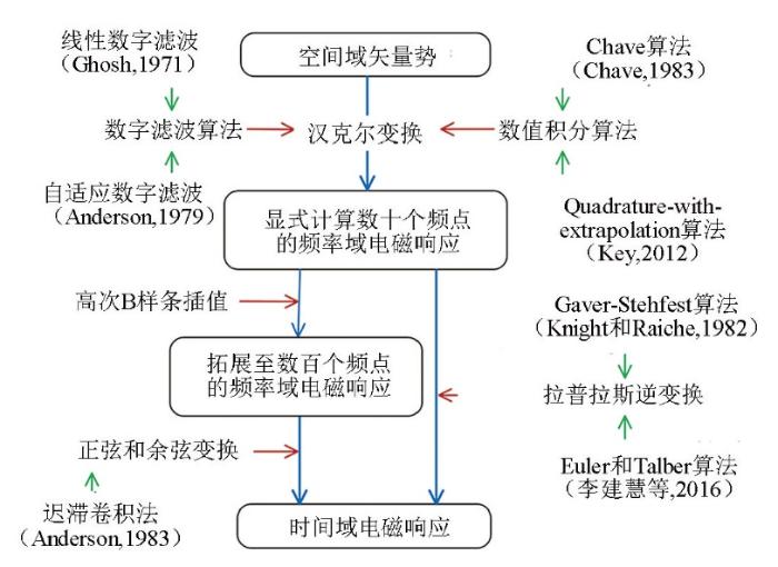
图1
瞬变电磁法一维正演技术路线
Fig.1
1D forward modeling technology roadmap for transient electromagnetic methods
式(2)中I为发射电流强度;a为圆形回线半径。
1.2 B样条插值函数
由于本文采用了Key研发的201个系数的正弦和余弦变换[9],需将上述显式计算的数十个频点的磁场频率域响应
其中:
1.3 时间域响应
将201个频点的磁场频率域响应通过正弦变换得到磁场脉冲响应数值解:
为了验证高次B样条插值效果,将上式得到的数值解与以下垂直磁偶源磁场脉冲响应的解析解(式(7))或圆形回线中心的磁场脉冲响应的解析解(式(8))对比。
其中:
2 算法验证
本文以垂直磁偶源和圆形回线源为例,验证高次B样条插值的效果。验证过程中用到3个评价标准:相对误差、最大相对误差和平均误差率,单位都为%。其中平均误差率是描述整个时间序列相对误差的一个量, n为时刻的数目。
设置观测时间序列共含30个时刻,其范围在10-5~10-1 s。通过试错法划定不同样条插值函数所需要的频率范围,传统三次样条频率范围为2π×10-1~2π×108 Hz,三次B样条频率范围为2π×10-2~2π×107 Hz,高次B样条频率范围统一划定为2π×10-3~2π×1013 Hz,每数量级的频点均为5。
2.1 垂直磁偶源
定义垂直磁偶源具有单位磁矩,收发距为100 m,均匀半空间电阻率为1 000 Ω·m。将图2a中垂直磁偶源的磁场频率域响应分别采用传统三次样条和三次B样条插值扩展,经正弦变换得到的磁场脉冲响应数值解都与解析解吻合良好。其中基于三次B样条插值和传统三次样条插值的最大相对误差均小于1.1%(图2b),基于五次B样条插值的最大相对误差小于0.06%(图2c),基于七次B样条插值的最大相对误差小于0.01%(图2d)。结果表明,垂直磁偶源位于1 000 Ω·m均匀半空间时,三次B样条和传统三次样条插值效果一致,五次和七次B样条插值效果远优于传统三次样条。同频点下,随着B样条阶次变高,最大相对误差减小,插值效果更优。
图2
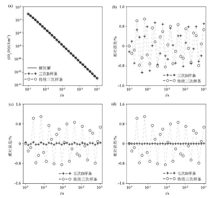
图2
每数量级5个频点计算条件下垂直磁偶源位于1 000 Ω·m均匀半空间表面激发的磁场脉冲响应
a—三次B样条数值解;b—三次B样条相对误差曲线;c—五次B样条相对误差曲线;d—七次B样条相对误差曲线
Fig.2
The magnetic field impulse response excited by vertical magnetic dipole source on the surface of 1 000 Ω·m homogeneous half-space on the condition of 5 frequencies per decade
a—cubic B-spline numerical solution;b—cubic B-spline relative error curve;c—quintic B-spline relative error curve;d—heptatic B-spline relative error curve
为探讨高次B样条的一般规律,给其阶次和每数量级频点的选择提供依据,在表1给出了垂直磁偶源位于1 000 Ω·m均匀半空间时,不同阶次B样条插值在每数量级不同频点情况下,正演计算产生的平均误差率,表2给出了最大相对误差。从整体上来看,平均误差率和最大相对误差都随着每数量级频点和B样条阶次的增加而减小。但该变化并不是线性的,例如七次B样条在每数量级频点为6时,其数值解的尾部出现了严重的震荡,导致平均误差率为265%,远大于附近频点和附近阶次B样条的平均误差率。经过分析,这种情况下B样条插值所需的约束范围更大,也就是所需的频率范围更大,而此时增大频率范围会导致划分的频点数过多, 影响正演效率,因此在选择插值方法时应当避开这些情况。因正演其他环节也会引起误差,且数值解与解析解本身存在一定的误差,经测试,平均误差率达到0.000 1%附近后不会再大幅减小。
表1 垂直磁偶源位于1 000 Ω·m均匀半空间时不同插值算法产生的平均误差率
Table 1
| 插值算法 | 平均误差率/% | |||||
|---|---|---|---|---|---|---|
| 4频点 | 5频点 | 6频点 | 7频点 | 8频点 | 9频点 | |
| 传统三次样条 | 9.08×10⁻¹ | 5.27×10⁻¹ | 3.75×10⁻¹ | 2.60×10⁻¹ | 3.21×10⁻¹ | 2.19×10⁻¹ |
| 三次B样条 | 9.11×10⁻¹ | 5.54×10⁻¹ | 3.68×10⁻¹ | 2.70×10⁻¹ | 3.10×10⁻¹ | 2.17×10⁻¹ |
| 四次B样条 | 7.20×10⁻¹ | 4.02×10³ | 1.50×10² | 1.00×101 | 6.22×10⁻² | 3.01×10⁻² |
| 五次B样条 | 6.53×10⁻² | 2.74×10⁻² | 1.28×10⁻² | 3.70×10⁻² | 5.71 | 6.31×101 |
| 六次B样条 | 1.03×10³ | 5.61×10⁻¹ | 4.46×10⁻³ | 2.03×10⁻³ | 1.65×10⁻³ | 1.29×10⁻³ |
| 七次B样条 | 1.53×10⁻² | 4.22×10⁻³ | 2.65×10² | 1.15 | 3.47×10⁻⁴ | 3.64×10⁻⁴ |
| 八次B样条 | 4.03×101 | 1.26 | 9.43×10⁻⁴ | 2.16×10⁻² | 1.08×10³ | 1.53 |
| 九次B样条 | 4.13 | 1.81×10⁻³ | 2.57×101 | 3.72×10⁻³ | 2.52×10⁻⁴ | 2.89×10⁻⁴ |
表2 垂直磁偶源位于1000 Ω·m均匀半空间时不同插值算法产生的最大相对误差
Table 2
| 插值算法 | 最大相对误差/% | |||||
|---|---|---|---|---|---|---|
| 4频点 | 5频点 | 6频点 | 7频点 | 8频点 | 9频点 | |
| 传统三次样条 | 1.81 | 1.09 | 7.24×10⁻¹ | 4.57×10⁻¹ | 6.98×10⁻¹ | 8.82×10⁻¹ |
| 三次B样条 | 1.93 | 1.06 | 6.89×10⁻¹ | 5.50×10⁻¹ | 6.66×10⁻¹ | 9.21×10⁻¹ |
| 四次B样条 | 1.38 | 2.60×10⁴ | 1.59×10³ | 1.12×10² | 6.56×10⁻¹ | 1.26×10⁻¹ |
| 五次B样条 | 1.31×10⁻¹ | 5.60×10⁻² | 2.50×10⁻² | 1.01×10⁻¹ | 2.17×101 | 5.25×10² |
| 六次B样条 | 5.19×10³ | 7.74 | 3.39×10⁻² | 1.17×10⁻² | 9.84×10⁻³ | 6.47×10⁻³ |
| 七次B样条 | 9.31×10⁻² | 1.08×10⁻² | 2.36×10³ | 1.35×101 | 1.62×10⁻³ | 1.81×10⁻³ |
| 八次B样条 | 1.48×10² | 1.82×101 | 1.47×10⁻² | 5.29×10⁻² | 9.53×10³ | 1.36×101 |
| 九次B样条 | 4.77×101 | 8.67×10⁻³ | 1.62×10² | 4.68×10⁻² | 5.12×10⁻³ | 2.08×10⁻³ |
验证B样条插值算法时也应考虑均匀半空间为低阻的极限情况,设置其电阻率为1 Ω·m,其余参数与电阻率为1 000 Ω·m时一致。图3a中的磁场脉冲响应数值解与解析解吻合良好。其中基于三次B样条插值和传统三次样条插值的最大相对误差小于4.2%(图3b),基于五次B样条插值的最大相对误差小于0.5%(图3c),基于七次B样条插值的最大相对误差小于0.4%(图3d),五次B样条和七次B样条插值效果差距不大。在图3a中0.002 s附近,垂直磁场变号,脉冲响应正负反转,导致样条插值在此处相对误差较大。结果表明:垂直磁偶源位于1 Ω·m均匀半空间时,拟合难度较大,高次B样条插值效果差于均匀半空间电阻率为1 000 Ω·m的情况。
图3
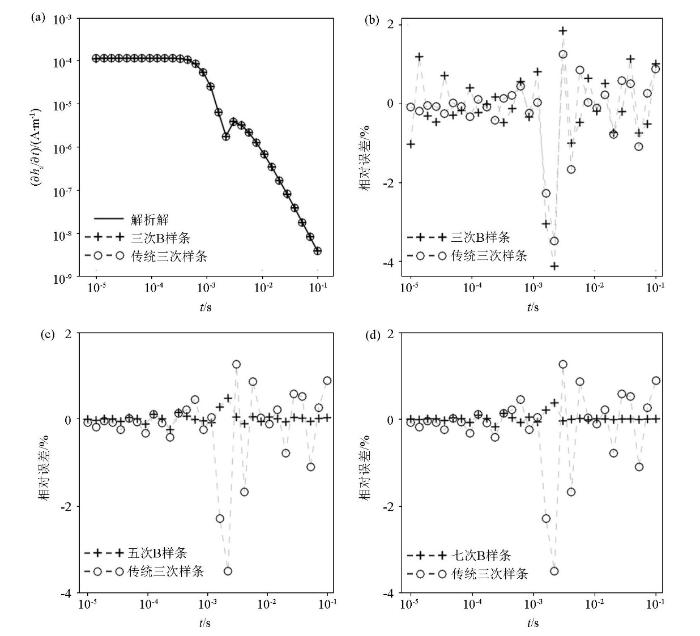
图3
每数量级5个频点计算条件下垂直磁偶源位于1 Ω·m均匀半空间表面激发的磁场脉冲响应
a—三次B样条数值解;b—三次B样条相对误差曲线;c—五次B样条相对误差曲线;d—七次B样条相对误差曲线
Fig.3
The magnetic field impulse response excited by the vertical magnetic dipole source on the surface of 1 Ω·m homogeneous half-space on the condition of 5 frequencies per decade
a—cubic B-spline numerical solution;b—cubic B-spline relative error curve;c—quintic B-spline relative error curve;d—heptatic B-spline relative error curve
表3 垂直磁偶源位于1 Ω·m均匀半空间时不同插值算法产生的平均误差率
Table 3
| 插值算法 | 平均误差率/% | |||||
|---|---|---|---|---|---|---|
| 4频点 | 5频点 | 6频点 | 7频点 | 8频点 | 9频点 | |
| 传统三次样条 | 1.71 | 5.59×10⁻¹ | 3.11×10⁻¹ | 1.82×10⁻¹ | 5.64×10⁻² | 5.69×10⁻² |
| 三次B样条 | 1.21×101 | 7.83×10⁻¹ | 3.16×10⁻¹ | 1.49×10⁻¹ | 7.80×10⁻² | 5.66×10⁻² |
| 四次B样条 | 4.76×10⁻¹ | 8.95 | 7.80×10⁻¹ | 1.03×10⁻¹ | 2.40×10⁻² | 1.42×10⁻² |
| 五次B样条 | 1.02 | 7.57×10⁻² | 3.21×10⁻² | 1.46×10⁻² | 1.07×10⁻² | 4.93×10⁻² |
| 六次B样条 | 4.31×101 | 1.08 | 3.12×10⁻² | 5.84×10⁻³ | 1.36×10⁻³ | 9.76×10⁻⁴ |
| 七次B样条 | 1.55 | 5.09×10⁻² | 1.33 | 2.11×10⁻² | 8.84×10⁻⁴ | 3.44×10⁻⁴ |
| 八次B样条 | 3.54 | 8.14×10⁻¹ | 1.09×10⁻² | 1.00×10⁻³ | 6.33×10⁻² | 4.56×10⁻⁴ |
| 九次B样条 | 8.00 | 3.74×10⁻² | 2.78×10⁻¹ | 1.13×10⁻³ | 2.54×10⁻⁴ | 4.82×10⁻⁵ |
表4 垂直磁偶源位于1 Ω·m均匀半空间时不同插值算法产生的最大相对误差
Table 4
| 插值算法 | 最大相对误差/% | |||||
|---|---|---|---|---|---|---|
| 4频点 | 5频点 | 6频点 | 7频点 | 8频点 | 9频点 | |
| 传统三次样条 | 4.85 | 3.49 | 2.63 | 1.37 | 2.35×10⁻¹ | 3.78×10⁻¹ |
| 三次B样条 | 1.08×10² | 4.13 | 2.32 | 1.54 | 4.11×10⁻¹ | 3.30×10⁻¹ |
| 四次B样条 | 3.87 | 1.32×10² | 8.80 | 6.70×10⁻¹ | 1.80×10⁻¹ | 9.19×10⁻² |
| 五次B样条 | 3.60 | 4.80×10⁻¹ | 2.02×10⁻¹ | 1.45×10⁻¹ | 8.59×10⁻² | 5.62×10⁻¹ |
| 六次B样条 | 6.46×10² | 8.81 | 1.80×10⁻¹ | 6.33×10⁻² | 8.03×10⁻³ | 9.17×10⁻³ |
| 七次B样条 | 8.70 | 3.74×10⁻¹ | 1.72×101 | 1.62×10⁻¹ | 6.13×10⁻³ | 3.09×10⁻³ |
| 八次B样条 | 4.44×101 | 6.69 | 3.85×10⁻² | 7.31×10⁻³ | 8.12×10⁻¹ | 3.63×10⁻³ |
| 九次B样条 | 8.02×101 | 1.72×10⁻¹ | 3.32 | 3.87×10⁻³ | 1.65×10⁻³ | 2.44×10⁻⁴ |
分析不同阶次的B样条插值的结果,为实现瞬变电磁响应的精确计算, 本文划定样条插值的平均误差率需小于0.1%,最大相对误差需小于1%。对于垂直磁偶源,满足条件的高次B样条有每数量级频点为5时,阶次为五次、七次和九次;每数量级频点为6时,阶次为五次、六次和八次;每数量级频点为7时,阶次为五次、六次、八次和九次;每数量级频点为8时,阶次为四次、六次、七次和九次;每数量级频点为9时,阶次为四次、六次、七次和九次。
2.2 圆形回线
圆形回线的参数设置如下:定义发射电流为1 A,回线半径为50 m,均匀半空间电阻率为1 000 Ω·m,测点位于回线中心。将图4a 中圆形回线中心磁场频率域响应分别采用传统三次样条和三次B样条插值扩展,经正弦变换得到的磁场脉冲响应数值解都与解析解吻合良好。其中基于传统三次样条插值的最大相对误差小于1.1%(图4b),基于三次B样条插值的最大相对误差小于2.9%(图4b),基于五次B样条插值的最大相对误差小于0.13%(图4c),基于七次B样条插值的最大相对误差小于0.15%(图4d)。基于七次B样条插值的晚期2个时刻相对误差较大,而其余时刻相对误差优于五次B样条。结果表明,圆形回线置于1 000 Ω·m均匀半空间时,传统三次样条插值效果较好,而随着B样条阶次变高,B样条插值的相对误差迅速下降,其插值效果反超传统三次样条。
图4
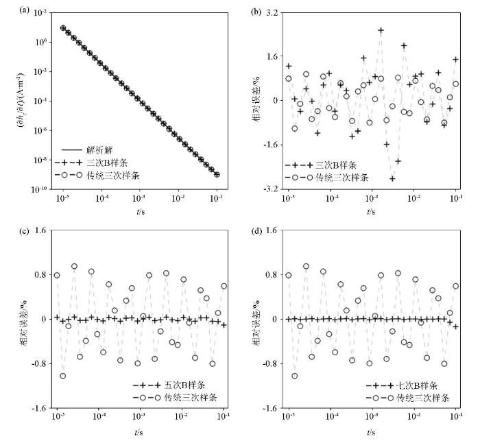
图4
每数量级5个频点计算条件下圆形回线位于1 000 Ω·m均匀半空间表面激发的磁场脉冲响应
a—三次B样条数值解;b—三次B样条相对误差曲线;c—五次B样条相对误差曲线;d—七次B样条相对误差曲线
Fig.4
The impulse response of magnetic field excited by circular loop on the surface of 1 000 Ω·m homogeneous half-space on the condition of 5 frequencied per decade
a—cubic B-spline numerical solution;b—cubic B-spline relative error curve;c—quintic B-spline relative error curve;d—heptatic B-spline relative error curve
表5 圆形回线位于1 000 Ω·m均匀半空间时不同插值算法产生的平均误差率
Table 5
| 插值算法 | 平均误差率/% | |||||
|---|---|---|---|---|---|---|
| 4频点 | 5频点 | 6频点 | 7频点 | 8频点 | 9频点 | |
| 传统三次样条 | 9.04×10⁻¹ | 5.41×10⁻¹ | 3.73×10⁻¹ | 3.18×10⁻¹ | 4.41×10⁻¹ | 1.86×10⁻¹ |
| 三次B样条 | 1.41 | 9.90×10⁻¹ | 8.59×10⁻¹ | 7.32×10⁻¹ | 8.65×10⁻¹ | 7.36×10⁻¹ |
| 四次B样条 | 2.83 | 6.24×10³ | 2.21×10³ | 1.28×10² | 2.92 | 4.89×10⁻² |
| 五次B样条 | 5.75×10⁻² | 2.77×10⁻² | 1.59×10⁻² | 4.41×10⁻¹ | 3.23×10² | 7.69×10⁴ |
| 六次B样条 | 4.25×10³ | 7.34 | 8.54×10⁻³ | 3.98×10⁻³ | 1.36×10⁻² | 4.44×10⁻³ |
| 七次B样条 | 1.99×10⁻² | 1.19×10⁻² | 3.45×10³ | 1.54×101 | 9.40×10⁻³ | 4.12×10⁻³ |
| 八次B样条 | 7.38×101 | 1.96×101 | 5.72×10⁻³ | 2.44×10⁻¹ | 7.07×10⁴ | 3.71×101 |
| 九次B样条 | 6.33 | 1.29×10⁻² | 4.33×10² | 4.77×10⁻² | 1.32×10⁻² | 5.25×10⁻³ |
表6 圆形回线位于1 000 Ω·m均匀半空间时不同插值算法产生的最大相对误差
Table 6
| 插值算法 | 最大相对误差/% | |||||
|---|---|---|---|---|---|---|
| 4频点 | 5频点 | 6频点 | 7频点 | 8频点 | 9频点 | |
| 传统三次样条 | 2.57 | 1.02 | 7.66×10⁻¹ | 5.90×10⁻¹ | 1.75 | 4.51×10⁻¹ |
| 三次B样条 | 7.46 | 2.82 | 2.86 | 2.92 | 2.41 | 2.47 |
| 四次B样条 | 5.16 | 4.05×10⁴ | 2.36×10⁴ | 1.46×10³ | 5.07×101 | 4.04×10⁻¹ |
| 五次B样条 | 1.17×10⁻¹ | 1.07×10⁻¹ | 7.81×10⁻² | 9.37×10⁻¹ | 1.34×10³ | 4.66×10⁵ |
| 六次B样条 | 2.06×10⁴ | 7.51×101 | 8.01×10⁻² | 7.54×10⁻² | 2.28×10⁻¹ | 4.39×10⁻² |
| 七次B样条 | 1.93×10⁻¹ | 1.35×10⁻¹ | 3.00×10⁴ | 1.92×10² | 1.62×10⁻¹ | 4.46×10⁻² |
| 八次B样条 | 2.92×10² | 1.98×10² | 7.46×10⁻² | 4.25×10⁻¹ | 6.04×10⁵ | 4.61×10² |
| 九次B样条 | 7.23×101 | 1.00×10⁻¹ | 5.02×10³ | 7.35×10⁻¹ | 2.34×10⁻¹ | 4.21×10⁻² |
图5
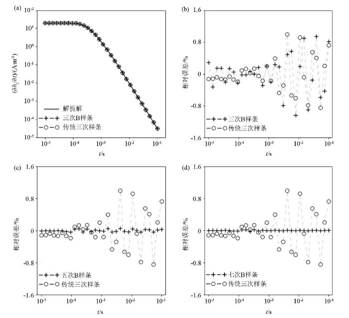
图5
每数量级5频点计算条件下圆形回线位于1 Ω·m均匀半空间表面激发的磁场脉冲响应
a—三次B样条数值解;b—三次B样条相对误差曲线;c—五次B样条相对误差曲线;d—七次B样条相对误差曲线
Fig.5
The impulse response of magnetic field excited by circular loop on the surface of 1 Ω·m homogeneous half-space on the condition of 5 frequencies per decade
a—cubic B-spline numerical solution;b—cubic B-spline relative error curve;c—quintic B-spline relative error curve;d—heptatic B-spline relative error curve
表7 圆形回线位于1 Ω·m均匀半空间时不同插值算法产生的平均误差率
Table 7
| 插值算法 | 平均误差率/% | |||||
|---|---|---|---|---|---|---|
| 4频点 | 5频点 | 6频点 | 7频点 | 8频点 | 9频点 | |
| 传统三次样条 | 6.14×10⁻¹ | 3.23×10⁻¹ | 2.07×10⁻¹ | 1.26×10⁻¹ | 1.21×10⁻¹ | 5.65×10⁻² |
| 三次B样条 | 1.02 | 3.55×10⁻¹ | 1.96×10⁻¹ | 1.26×10⁻¹ | 1.17×10⁻¹ | 5.67×10⁻² |
| 四次B样条 | 1.45×10⁻¹ | 2.81×10⁻¹ | 4.03×10⁻² | 2.19×10⁻² | 1.70×10⁻² | 7.16×10⁻³ |
| 五次B样条 | 1.75×10⁻¹ | 2.46×10⁻² | 1.05×10⁻² | 4.96×10⁻³ | 6.48×10⁻³ | 7.58×10⁻² |
| 六次B样条 | 2.07 | 4.60×10⁻² | 4.76×10⁻³ | 1.42×10⁻³ | 7.26×10⁻⁴ | 2.12×10⁻⁴ |
| 七次B样条 | 1.84×10⁻¹ | 6.60×10⁻³ | 1.54×10⁻² | 1.62×10⁻³ | 2.52×10⁻⁴ | 6.78×10⁻⁵ |
| 八次B样条 | 1.15×10⁻¹ | 3.40×10⁻² | 1.22×10⁻³ | 2.43×10⁻⁴ | 5.44×10⁻² | 3.00×10⁻⁵ |
| 九次B样条 | 3.25×10⁻¹ | 5.25×10⁻³ | 8.17×10⁻⁴ | 4.29×10⁻⁴ | 4.50×10⁻⁵ | 1.08×10⁻⁵ |
表8 圆形回线位于1 Ω·m均匀半空间时不同插值算法产生的最大相对误差
Table 8
| 插值算法 | 最大相对误差/% | |||||
|---|---|---|---|---|---|---|
| 4频点 | 5频点 | 6频点 | 7频点 | 8频点 | 9频点 | |
| 传统三次样条 | 1.88 | 9.94×10⁻¹ | 6.83×10⁻¹ | 4.15×10⁻¹ | 5.90×10⁻¹ | 2.82×10⁻¹ |
| 三次B样条 | 5.34 | 1.03 | 7.21×10⁻¹ | 4.86×10⁻¹ | 5.75×10⁻¹ | 2.50×10⁻¹ |
| 四次B样条 | 3.57×10⁻¹ | 3.29 | 1.09×10⁻¹ | 5.52×10⁻² | 6.24×10⁻² | 3.16×10⁻² |
| 五次B样条 | 6.67×10⁻¹ | 5.16×10⁻² | 2.52×10⁻² | 1.02×10⁻² | 6.00×10⁻² | 8.42×10⁻¹ |
| 六次B样条 | 2.65×101 | 3.43×10⁻¹ | 1.40×10⁻² | 2.55×10⁻³ | 2.22×10⁻³ | 9.95×10⁻⁴ |
| 七次B样条 | 1.16 | 2.72×10⁻² | 1.81×10⁻¹ | 1.07×10⁻² | 5.10×10⁻⁴ | 2.07×10⁻⁴ |
| 八次B样条 | 1.15 | 2.93×10⁻¹ | 7.41×10⁻³ | 1.08×10⁻³ | 6.67×10⁻¹ | 8.09×10⁻⁵ |
| 九次B样条 | 3.41 | 3.01×10⁻² | 5.73×10⁻³ | 1.91×10⁻³ | 1.64×10⁻⁴ | 3.27×10⁻⁵ |
对于圆形回线源,满足本文划定精确计算要求的高次B样条有每数量级频点为5时,阶次为五次、七次和九次;每数量级频点为6时,阶次为五次、六次和八次;每数量级频点为7时,阶次为六次和九次;每数量级频点为8时,阶次为六次、七次和九次;每数量级频点为9时,阶次为四次、六次、七次和九次。
综合2种发射源布置在不同地电模型的结果来看,高次B样条的平均误差率和最大相对误差随频点的变化不稳定,但是经过对比,满足瞬变电磁响应精确计算的几种插值算法所需频点和阶次是固定的。归纳总结的结果满足本文划定精确计算要求,且适用于不同发射源的高次B样条插值算法。归纳结果与圆形回线源划定的高次B样条一致,此处不再复述。在兼顾瞬变电磁响应高精度计算要求和正演效率的前提下,选择五次、七次或九次B样条在每数量级频点为5时插值最合理,此时频点划分个数为81。九次B样条在每数量级频点为9时进行插值的平均误差率和最大相对误差最小,之后再增加阶次和频点,误差也不会大幅减小,推测此时一维正演其他环节引起的误差掩盖了B样条阶次和频点继续增加所带来的误差变化。
3 结论
本文将高次B样条插值应用瞬变电磁法一维正演中,并以垂直磁偶源和圆形回线源为例,验证了算法的准确性。数值结果表明,对于多个地电模型,基于高次B样条插值计算的瞬变电磁响应精度均优于基于传统三次样条的计算结果。其中五次、七次或九次B样条在每数量级频点为5时插值效果既满足瞬变电磁响应高精度计算的要求,又可以兼顾正演效率。
参考文献
瞬变电磁法勘探的地电模型及其成功案例分析
[J].
Geoelectric models and their corresponding successful cases for transient electromagnetic prospecting
[J].
Effects of full transmitting-current waveforms on transient electromagnetics:Insights from modeling the Albany graphite deposit
[J].
DOI:10.1190/geo2018-0573.1
URL
[本文引用: 1]

In transient electromagnetic (TEM) methods, the full transmitting-current waveform, not just the abrupt turn-off, can have effects on the measured responses. A 3D finite-element time-domain forward-modeling solver was used to investigate these effects. This was motivated by an attempt to match, via forward-modeling, real data from the Albany graphite deposit in northern Ontario, Canada. Initial modeling results for homogeneous half-spaces illustrate the effects that a full waveform can have on TEM responses, especially the durations of the steady stage and turn-off time. For the Albany data set, a geophysical conductivity model was developed from a geologic model that itself had been constructed predominantly from drillhole information. The conductivities of the various geologic units in the model were first estimated based on typical conductivity values for the respective rock types, then adjusted to fit the measured TEM data as closely as possible. We found that the TEM responses differed significantly from the pure step-off response and that incorporating the effects of the full waveform (particularly the linear ramp turn-off) greatly improved the match between observed and computed responses, especially for the early measurement times. In addition, this Albany example illustrates the presence of sign changes in TEM data caused primarily by localized conductivity targets.
TDEM survey in urban environmental for hydrogeological study at USP campus in So Paulo city,Brazil
[J].DOI:10.1016/j.jappgeo.2011.10.001 URL [本文引用: 1]
瞬变电磁法正演计算进展
[J].
Progress of forward computation in transient electromagnetic method
[J].
回线源瞬变电磁法的一维Occam反演
[J].
One-dimensional Occam ‘s inversion for transient electromagnetic data excited by a loop source
[J].
The application of linear filter theory to the direct interpretation of geoelectrical resistivity sounding measurements
[J].DOI:10.1111/gpr.1971.19.issue-2 URL [本文引用: 1]
Computer program numerical integration of related Hankel transforms of orders 0 and 1 by adaptive digital filtering
[J].
DOI:10.1190/1.1441007
URL
[本文引用: 1]
A linear digital filtering algorithm is presented for rapid and accurate numerical evaluation of Hankel transform integrals of orders 0 and 1 containing related complex kernel functions. The kernel for Hankel transforms is defined as the non‐Bessel function factor of the integrand. Related transforms are defined as transforms, of either order 0 or 1, whose kernel functions are related to one another by simple algebraic relationships. Previously saved kernel evaluations are used in the algorithm to obtain rapidly either order transform following an initial convolution operation. Each order filter is designed with identical abscissas over a large range so that an adaptive convolution procedure can be applied to a large class of kernels. Different order Hankel transforms with related kernels are often found in electromagnetic (EM) applications. Because of the general nature of this algorithm, the need to design new filters should not be necessary for most applications. Accuracy of the filters is comparable to that of single‐precision numerical quadrature methods, provided well‐behaved kernels and moderate values of the transform argument are used. Filtering errors of less than 0.005 percent are demonstrated numerically using known analytical Hankel transform pairs. The digital filter accuracy is also illustrated by comparison with other published filters for computing the apparent resistivity for a Schlumberger array over a horizontally layered earth model. The algorithm is written in Fortran IV and is listed in the Appendix along with a test driver program. Detailed comments are included to define sufficiently all calling parameter requirements.
Numerical integration of related Hankel transforms by quadrature and continued fraction expansion
[J].
DOI:10.1190/1.1441448
URL
[本文引用: 1]
An algorithm is presented for the accurate evaluation of Hankel (or Bessel) transforms of algebraically related kernel functions, defined here as the non‐Bessel function portion of the integrand, that is more widely applicable than the standard digital filter methods without enormous increases in computational burden. The algorithm performs the automatic integration of the product of the kernel and Bessel functions between the asymptotic zero crossings of the latter and sums the series of partial integrations using a continued fraction expansion, equivalent to an analytic continuation of the series. The integrands may be saved to allow the rapid computation of related transforms without recalculating the kernel or Bessel functions, and the integration steps use interlacing quadrature formulas so that no function evaluations are wasted when it is necessary to increase the order of the quadrature rule. The continued fraction algorithm allows very slowly divergent or even formally divergent integrals to be computed quite easily. The local error is controlled at each step in the algorithm, and accuracy is limited largely by machine resolution. The algorithm is written in Fortran and is listed in an Appendix along with a driver program that illustrates its features. The driver program and subroutine are available from the SEG Business Office.
Is the fast Hankel transform faster than quadrature
?[J].
DOI:10.1190/geo2011-0237.1
URL
[本文引用: 2]
The fast Hankel transform (FHT) implemented with digital filters has been the algorithm of choice in EM geophysics for a few decades. However, other disciplines have predominantly relied on methods that break up the Hankel transform integral into a sum of partial integrals that are each evaluated with quadrature. The convergence of the partial sums is then accelerated through a nonlinear sequence transformation. While such a method was proposed for geophysics nearly three decades ago, it was demonstrated to be much slower than the FHT. This work revisits this problem by presenting a new algorithm named quadrature-with-extrapolation (QWE). The QWE method recasts the quadrature sum into a form conceptually similar to the FHT approach by using a fixed-point quadrature rule. The sum of partial integrals is efficiently accelerated using the Shanks transformation computed with Wynn’s [Formula: see text] algorithm. A Matlab implementation of the QWE algorithm is compared with the FHT method for accuracy and speed on a suite of relevant modeling problems including frequency-domain controlled-source EM, time-domain EM, and a large-loop magnetic source problem. Surprisingly, the QWE method is faster than the FHT for all three problems. However, when the integral needs to be evaluated at many offsets and the lagged convolution variant of the FHT is applicable, the FHT is significantly faster than the QWE method. For divergent integrals such as those encountered in the large loop problem, the QWE method can provide an accurate answer when the FHT method fails.
Fourier cosine and sine transforms using lagged convolutions in double-precision(subprograms DLAGF0/DLAGF1)
[R].
A hybrid fast Hankel transform algorithm for electromagnetic modeling
[J].
DOI:10.1190/1.1442650
URL
[本文引用: 1]
A hybrid fast Hankel transform algorithm has been developed that uses several complementary features of two existing algorithms: Anderson’s digital filtering or fast Hankel transform (FHT) algorithm and Chave’s quadrature and continued fraction algorithm. A hybrid FHT subprogram (called HYBFHT) written in standard Fortran-77 provides a simple user interface to call either subalgorithm. The hybrid approach is an attempt to combine the best features of the two subalgorithms in order to minimize the user’s coding requirements and to provide fast execution and good accuracy for a large class of electromagnetic problems involving various related Hankel transform sets with multiple arguments. Special cases of Hankel transforms of double‐order and double‐argument are discussed, where use of HYBFHT is shown to be advantageous for oscillatory kernel functions.
Transient electromagnetic calculations using the Gaver-Stehfest inverse Laplace transform method
[J].
DOI:10.1190/1.1441280
URL
[本文引用: 1]
Calculations for the transient electromagnetic (TEM) method are commonly performed by using a discrete Fourier transform method to invert the appropriate transform of the solution. We derive the Laplace transform of the solution for TEM soundings over an N‐layer earth and show how to use the Gaver‐Stehfest algorithm to invert it numerically. This is considerably more stable and computationally efficient than inversion using the discrete Fourier transform.
Three effective inverse Laplace transform algorithms for computing time-domain electromagnetic responses
[J].
DOI:10.1190/geo2015-0174.1
URL
[本文引用: 1]
The inverse Laplace transform is one of the methods used to obtain time-domain electromagnetic (EM) responses in geophysics. The Gaver-Stehfest algorithm has so far been the most popular technique to compute the Laplace transform in the context of transient electromagnetics. However, the accuracy of the Gaver-Stehfest algorithm, even when using double-precision arithmetic, is relatively low at late times due to round-off errors. To overcome this issue, we have applied variable-precision arithmetic in the MATLAB computing environment to an implementation of the Gaver-Stehfest algorithm. This approach has proved to be effective in terms of improving accuracy, but it is computationally expensive. In addition, the Gaver-Stehfest algorithm is significantly problem dependent. Therefore, we have turned our attention to two other algorithms for computing inverse Laplace transforms, namely, the Euler and Talbot algorithms. Using as examples the responses for central-loop, fixed-loop, and horizontal electric dipole sources for homogeneous and layered mediums, these two algorithms, implemented using normal double-precision arithmetic, have been shown to provide more accurate results and to be less problem dependent than the standard Gaver-Stehfest algorithm. Furthermore, they have the capacity for yielding more accurate time-domain responses than the cosine and sine transforms for which the frequency-domain responses are obtained by interpolation between a limited number of explicitly computed frequency-domain responses. In addition, the Euler and Talbot algorithms have the potential of requiring fewer Laplace- or frequency-domain function evaluations than do the other transform methods commonly used to compute time-domain EM responses, and thus of providing a more efficient option.
Contributions to the problem of approximation of equidistant data by analytic functions
[J].DOI:10.1090/qam/1946-04-01 URL [本文引用: 1]
On calculating with B-splines
[J].DOI:10.1016/0021-9045(72)90080-9 URL [本文引用: 1]
The Numerical evaluation of B-splines
[J].DOI:10.1093/imamat/10.2.134 URL [本文引用: 1]
B样条曲线生成原理及实现
[J].
The creating principle and realization of B-spline curve
[J].
A least-squares smooth fitting for irregularly spaced data:Finite-element approach using the cubic B-spline basis
[J].
DOI:10.1190/1.1442060
URL
[本文引用: 1]
A new method of multivariate smooth fitting of scattered, noisy data using cubic B-splines was developed. An optimum smoothing function was defined to minimize the [Formula: see text] norm composed of the data residuals and the first and the second derivatives, which represent the total misfit, fluctuation, and roughness of the function, respectively. The function is approximated by a cubic B‐spline expansion with equispaced knots. The solution can be interpreted in three ways. From the stochastic viewpoint, it is the maximum‐likelihood estimate among the admissible functions under the a priori information that the first and second derivatives are zero everywhere due to random errors, i.e., white noise. From the physical viewpoint, it is the finite‐element approximation for a lateral displacement of a bar or a plate under tension which is pulled to the data points by springs. From a technical viewpoint, it is an improved spline‐fitting algorithm. The additional condition of minimizing the derivative norms stabilizes the linear equation system for the expansion coefficients.
瞬变电磁测深的微分电导成像
[J].
Differential coefficient imaging of the longitudinal conductance in the transient electromagnetic sounding
[J].
Time-domain integral equation solvers using quadratic B-spline temporal basis functions
[J].DOI:10.1002/(ISSN)1098-2760 URL [本文引用: 1]
区间B样条小波有限元GPR模拟双相随机混凝土介质
[J].
The GPR simulation of bi-phase random concrete medium using finite element of B-spline wavelet on the interval
[J].
3D Wavelet finite-element modeling of frequency-domain airborne EM data based on B-spline wavelet on the interval using potentials
[J].
DOI:10.3390/rs13173463
URL
[本文引用: 1]
We present a wavelet finite-element method (WFEM) based on B-spline wavelets on the interval (BSWI) for three-dimensional (3D) frequency-domain airborne EM modeling using a secondary coupled-potential formulation. The BSWI, which is constructed on the interval (0, 1) by joining piecewise B-spline polynomials between nodes together, has proved to have excellent numerical properties of multiresolution and sparsity and thus is utilized as the basis function in our WFEM. Compared to conventional basis functions, the BSWI is able to provide higher interpolating accuracy and boundary stability. Furthermore, due to the sparsity of the wavelet, the coefficient matrix obtained by BSWI-based WFEM is sparser than that formed by general FEM, which can lead to shorter solution time for the linear equations system. To verify the accuracy and efficiency of our proposed method, we ran numerical experiments on a half-space model and a layered model and compared the results with one-dimensional (1D) semi-analytic solutions and those obtained from conventional FEM. We then studied a synthetic 3D model using different meshes and BSWI basis at different scales. The results show that our method depends less on the mesh, and the accuracy can be improved by both mesh refinement and scale enhancement.
Suppressing the very low-frequency noise by B-spline gating of transient electromagnetic data
[J].
DOI:10.1093/jge/gxac049
URL
[本文引用: 1]
Very low-frequency (VLF) communication signals of 15–25 kHz contaminate the transient electromagnetic (TEM) data. The notch filter or Butterworth filter is commonly used to suppress VLF noise in addition to synchronous detection of TEM data such as gating and stacking, while also introducing the TEM signal distortion around the VLF band. We propose a B-spline gating, which suppresses the VLF noise while integrating TEM data in the gate interval without any extra filter. B-spline gating is designed to ensure that the zeros of its amplitude frequency response (AFR) are located around VLF frequencies by optimizing the knot vector of the B-spline. It is available for various VLF frequencies. We apply B-spline gating to synthetic TEM data compared with rectangular gating and full-tapered gating, the AFRs of B-spline and full-tapered gating are 25 dB lower at high frequencies than rectangular gating, and the amplitude of B-spline is more reduced at VLF frequency than full-tapered gating; the standard error of the B-spline gates is reduced by >15% compared to the full-tapered gates. The field example from a TEM survey in the Inner Mongolia Autonomous Region of China shows that the amplitude of B-spline gating frequency response in late gates is reduced by about 20 dB at 24.1 kHz VLF than that of full-tapered gating, and the standard error is lower. It is concluded that B-spline gating can suppress VLF noise while following the normal decay of TEM signal without distortion.
