|
|
|
| One-dimensional accurate calculation of transient electromagnetic responses based on B-spline interpolation |
XING Tao1( ), WANG Yao2, LI Jian-Hui2,3() ), WANG Yao2, LI Jian-Hui2,3() |
1. Beijing Tanchuang Resources Technology Co., Ltd., Beijing 100071, China
2. School of Geophysics and Geomatics, China University of Geosciences (Wuhan), Wuhan 430074, China
3. State Key Laboratory of Geological Processes and Mineral Resources, China University of Geosciences (Wuhan), Wuhan 430074, China |
|
|
|
|
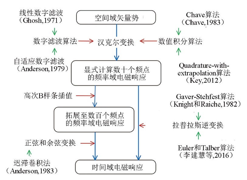
Abstract In the one-dimensional (1D) forward modeling of transient electromagnetic (TEM) responses based on spectral methods, multiple calculation steps significantly influence the calculation accuracy of TEM responses. To improve the efficiency of 1D forward modeling, the common practice is to directly calculate the frequency-domain electromagnetic responses of dozens of frequency points and then obtain the responses of hundreds of frequency points through cubic spline interpolation. Although the numerical results calculated using the cubic spline interpolation function can meet the requirements of most forward modeling scenarios, their accuracy can be further improved. This study introduced high-order B-spline interpolation into the 1D forward modeling of TEM responses to replace the conventional cubic spline interpolation and verified the accuracy of the method based on magnetic dipole sources and circle-shaped loop sources. The results show that the TEM responses of several geoelectric models calculated based on high-order B-spline interpolation exhibit higher accuracy than those calculated using conventional cubic spline interpolation.
|
|
Received: 09 December 2022
Published: 27 October 2023
|
|
|
|
Corresponding Authors:
LI Jian-Hui
E-mail: 156663062@qq.com;ljhiicumt@126.com
|
|
|
|
|
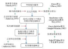
1D forward modeling technology roadmap for transient electromagnetic methods
|
|
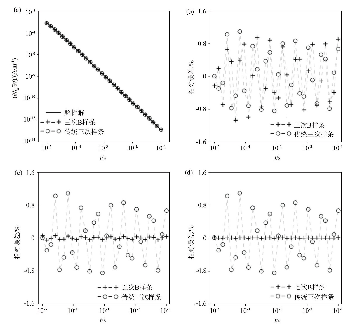
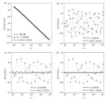
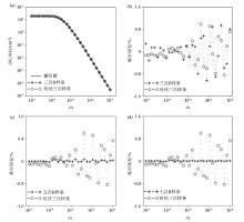
The magnetic field impulse response excited by vertical magnetic dipole source on the surface of 1 000 Ω·m homogeneous half-space on the condition of 5 frequencies per decade
a—cubic B-spline numerical solution;b—cubic B-spline relative error curve;c—quintic B-spline relative error curve;d—heptatic B-spline relative error curve
|

| 插值算法 | 平均误差率/% | | 4频点 | 5频点 | 6频点 | 7频点 | 8频点 | 9频点 | | 传统三次样条 | 9.08×10⁻¹ | 5.27×10⁻¹ | 3.75×10⁻¹ | 2.60×10⁻¹ | 3.21×10⁻¹ | 2.19×10⁻¹ | | 三次B样条 | 9.11×10⁻¹ | 5.54×10⁻¹ | 3.68×10⁻¹ | 2.70×10⁻¹ | 3.10×10⁻¹ | 2.17×10⁻¹ | | 四次B样条 | 7.20×10⁻¹ | 4.02×10³ | 1.50×10² | 1.00×101 | 6.22×10⁻² | 3.01×10⁻² | | 五次B样条 | 6.53×10⁻² | 2.74×10⁻² | 1.28×10⁻² | 3.70×10⁻² | 5.71 | 6.31×101 | | 六次B样条 | 1.03×10³ | 5.61×10⁻¹ | 4.46×10⁻³ | 2.03×10⁻³ | 1.65×10⁻³ | 1.29×10⁻³ | | 七次B样条 | 1.53×10⁻² | 4.22×10⁻³ | 2.65×10² | 1.15 | 3.47×10⁻⁴ | 3.64×10⁻⁴ | | 八次B样条 | 4.03×101 | 1.26 | 9.43×10⁻⁴ | 2.16×10⁻² | 1.08×10³ | 1.53 | | 九次B样条 | 4.13 | 1.81×10⁻³ | 2.57×101 | 3.72×10⁻³ | 2.52×10⁻⁴ | 2.89×10⁻⁴ |
|
Average error rate of different interpolation algorithms for a vertical magnetic dipole source in a 1000 Ω·m uniform half-space
|
| 插值算法 | 最大相对误差/% | | 4频点 | 5频点 | 6频点 | 7频点 | 8频点 | 9频点 | | 传统三次样条 | 1.81 | 1.09 | 7.24×10⁻¹ | 4.57×10⁻¹ | 6.98×10⁻¹ | 8.82×10⁻¹ | | 三次B样条 | 1.93 | 1.06 | 6.89×10⁻¹ | 5.50×10⁻¹ | 6.66×10⁻¹ | 9.21×10⁻¹ | | 四次B样条 | 1.38 | 2.60×10⁴ | 1.59×10³ | 1.12×10² | 6.56×10⁻¹ | 1.26×10⁻¹ | | 五次B样条 | 1.31×10⁻¹ | 5.60×10⁻² | 2.50×10⁻² | 1.01×10⁻¹ | 2.17×101 | 5.25×10² | | 六次B样条 | 5.19×10³ | 7.74 | 3.39×10⁻² | 1.17×10⁻² | 9.84×10⁻³ | 6.47×10⁻³ | | 七次B样条 | 9.31×10⁻² | 1.08×10⁻² | 2.36×10³ | 1.35×101 | 1.62×10⁻³ | 1.81×10⁻³ | | 八次B样条 | 1.48×10² | 1.82×101 | 1.47×10⁻² | 5.29×10⁻² | 9.53×10³ | 1.36×101 | | 九次B样条 | 4.77×101 | 8.67×10⁻³ | 1.62×10² | 4.68×10⁻² | 5.12×10⁻³ | 2.08×10⁻³ |
|
Maximum relative error of different interpolation algorithms for a vertical magnetic dipole source in a 1000 Ω·m uniform half-space
|
|
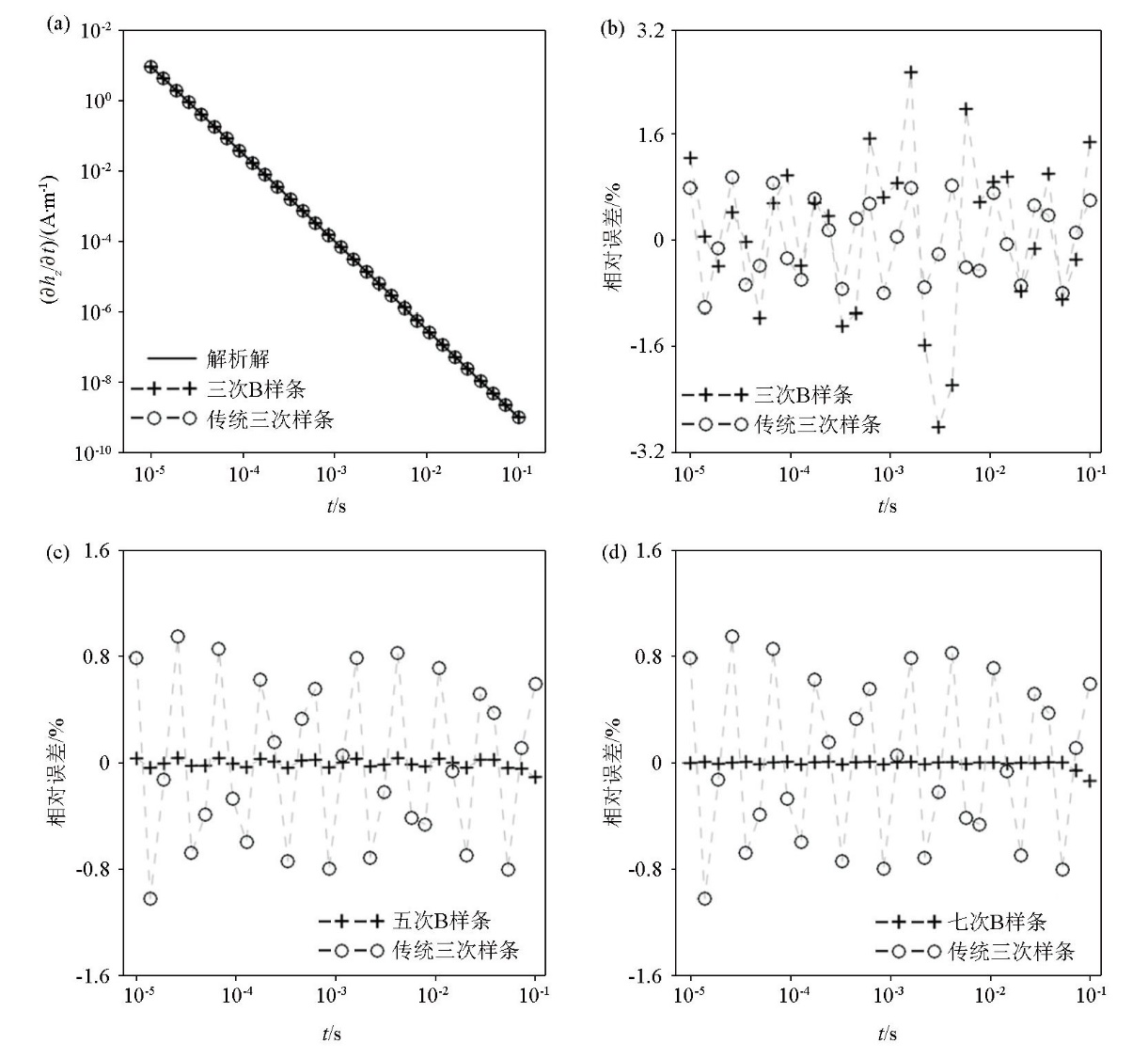
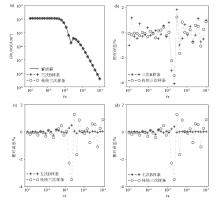
The magnetic field impulse response excited by the vertical magnetic dipole source on the surface of 1 Ω·m homogeneous half-space on the condition of 5 frequencies per decade
a—cubic B-spline numerical solution;b—cubic B-spline relative error curve;c—quintic B-spline relative error curve;d—heptatic B-spline relative error curve
|
| 插值算法 | 平均误差率/% | | 4频点 | 5频点 | 6频点 | 7频点 | 8频点 | 9频点 | | 传统三次样条 | 1.71 | 5.59×10⁻¹ | 3.11×10⁻¹ | 1.82×10⁻¹ | 5.64×10⁻² | 5.69×10⁻² | | 三次B样条 | 1.21×101 | 7.83×10⁻¹ | 3.16×10⁻¹ | 1.49×10⁻¹ | 7.80×10⁻² | 5.66×10⁻² | | 四次B样条 | 4.76×10⁻¹ | 8.95 | 7.80×10⁻¹ | 1.03×10⁻¹ | 2.40×10⁻² | 1.42×10⁻² | | 五次B样条 | 1.02 | 7.57×10⁻² | 3.21×10⁻² | 1.46×10⁻² | 1.07×10⁻² | 4.93×10⁻² | | 六次B样条 | 4.31×101 | 1.08 | 3.12×10⁻² | 5.84×10⁻³ | 1.36×10⁻³ | 9.76×10⁻⁴ | | 七次B样条 | 1.55 | 5.09×10⁻² | 1.33 | 2.11×10⁻² | 8.84×10⁻⁴ | 3.44×10⁻⁴ | | 八次B样条 | 3.54 | 8.14×10⁻¹ | 1.09×10⁻² | 1.00×10⁻³ | 6.33×10⁻² | 4.56×10⁻⁴ | | 九次B样条 | 8.00 | 3.74×10⁻² | 2.78×10⁻¹ | 1.13×10⁻³ | 2.54×10⁻⁴ | 4.82×10⁻⁵ |
|
Average error rate of different interpolation algorithms for a vertical magnetic dipole source in a 1 Ω·m uniform half-space
|
| 插值算法 | 最大相对误差/% | | 4频点 | 5频点 | 6频点 | 7频点 | 8频点 | 9频点 | | 传统三次样条 | 4.85 | 3.49 | 2.63 | 1.37 | 2.35×10⁻¹ | 3.78×10⁻¹ | | 三次B样条 | 1.08×10² | 4.13 | 2.32 | 1.54 | 4.11×10⁻¹ | 3.30×10⁻¹ | | 四次B样条 | 3.87 | 1.32×10² | 8.80 | 6.70×10⁻¹ | 1.80×10⁻¹ | 9.19×10⁻² | | 五次B样条 | 3.60 | 4.80×10⁻¹ | 2.02×10⁻¹ | 1.45×10⁻¹ | 8.59×10⁻² | 5.62×10⁻¹ | | 六次B样条 | 6.46×10² | 8.81 | 1.80×10⁻¹ | 6.33×10⁻² | 8.03×10⁻³ | 9.17×10⁻³ | | 七次B样条 | 8.70 | 3.74×10⁻¹ | 1.72×101 | 1.62×10⁻¹ | 6.13×10⁻³ | 3.09×10⁻³ | | 八次B样条 | 4.44×101 | 6.69 | 3.85×10⁻² | 7.31×10⁻³ | 8.12×10⁻¹ | 3.63×10⁻³ | | 九次B样条 | 8.02×101 | 1.72×10⁻¹ | 3.32 | 3.87×10⁻³ | 1.65×10⁻³ | 2.44×10⁻⁴ |
|
Maximum relative error of different interpolation algorithms for a vertical magnetic dipole source in a 1 Ω·m uniform half-space
|
|
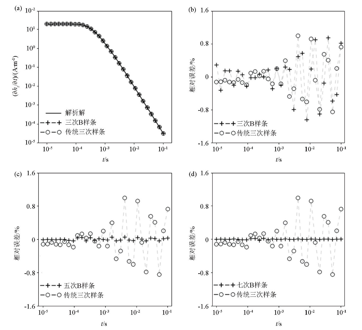
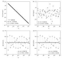
The impulse response of magnetic field excited by circular loop on the surface of 1 000 Ω·m homogeneous half-space on the condition of 5 frequencied per decade
a—cubic B-spline numerical solution;b—cubic B-spline relative error curve;c—quintic B-spline relative error curve;d—heptatic B-spline relative error curve
|
| 插值算法 | 平均误差率/% | | 4频点 | 5频点 | 6频点 | 7频点 | 8频点 | 9频点 | | 传统三次样条 | 9.04×10⁻¹ | 5.41×10⁻¹ | 3.73×10⁻¹ | 3.18×10⁻¹ | 4.41×10⁻¹ | 1.86×10⁻¹ | | 三次B样条 | 1.41 | 9.90×10⁻¹ | 8.59×10⁻¹ | 7.32×10⁻¹ | 8.65×10⁻¹ | 7.36×10⁻¹ | | 四次B样条 | 2.83 | 6.24×10³ | 2.21×10³ | 1.28×10² | 2.92 | 4.89×10⁻² | | 五次B样条 | 5.75×10⁻² | 2.77×10⁻² | 1.59×10⁻² | 4.41×10⁻¹ | 3.23×10² | 7.69×10⁴ | | 六次B样条 | 4.25×10³ | 7.34 | 8.54×10⁻³ | 3.98×10⁻³ | 1.36×10⁻² | 4.44×10⁻³ | | 七次B样条 | 1.99×10⁻² | 1.19×10⁻² | 3.45×10³ | 1.54×101 | 9.40×10⁻³ | 4.12×10⁻³ | | 八次B样条 | 7.38×101 | 1.96×101 | 5.72×10⁻³ | 2.44×10⁻¹ | 7.07×10⁴ | 3.71×101 | | 九次B样条 | 6.33 | 1.29×10⁻² | 4.33×10² | 4.77×10⁻² | 1.32×10⁻² | 5.25×10⁻³ |
|
Average error rate of different interpolation algorithms for circular loops in 1 000 Ω·m uniform half-space
|
| 插值算法 | 最大相对误差/% | | 4频点 | 5频点 | 6频点 | 7频点 | 8频点 | 9频点 | | 传统三次样条 | 2.57 | 1.02 | 7.66×10⁻¹ | 5.90×10⁻¹ | 1.75 | 4.51×10⁻¹ | | 三次B样条 | 7.46 | 2.82 | 2.86 | 2.92 | 2.41 | 2.47 | | 四次B样条 | 5.16 | 4.05×10⁴ | 2.36×10⁴ | 1.46×10³ | 5.07×101 | 4.04×10⁻¹ | | 五次B样条 | 1.17×10⁻¹ | 1.07×10⁻¹ | 7.81×10⁻² | 9.37×10⁻¹ | 1.34×10³ | 4.66×10⁵ | | 六次B样条 | 2.06×10⁴ | 7.51×101 | 8.01×10⁻² | 7.54×10⁻² | 2.28×10⁻¹ | 4.39×10⁻² | | 七次B样条 | 1.93×10⁻¹ | 1.35×10⁻¹ | 3.00×10⁴ | 1.92×10² | 1.62×10⁻¹ | 4.46×10⁻² | | 八次B样条 | 2.92×10² | 1.98×10² | 7.46×10⁻² | 4.25×10⁻¹ | 6.04×10⁵ | 4.61×10² | | 九次B样条 | 7.23×101 | 1.00×10⁻¹ | 5.02×10³ | 7.35×10⁻¹ | 2.34×10⁻¹ | 4.21×10⁻² |
|
Maximum relative error of different interpolation algorithms for circular loops in 1 000 Ω·m uniform half-space
|
|
The impulse response of magnetic field excited by circular loop on the surface of 1 Ω·m homogeneous half-space on the condition of 5 frequencies per decade
a—cubic B-spline numerical solution;b—cubic B-spline relative error curve;c—quintic B-spline relative error curve;d—heptatic B-spline relative error curve
|
| 插值算法 | 平均误差率/% | | 4频点 | 5频点 | 6频点 | 7频点 | 8频点 | 9频点 | | 传统三次样条 | 6.14×10⁻¹ | 3.23×10⁻¹ | 2.07×10⁻¹ | 1.26×10⁻¹ | 1.21×10⁻¹ | 5.65×10⁻² | | 三次B样条 | 1.02 | 3.55×10⁻¹ | 1.96×10⁻¹ | 1.26×10⁻¹ | 1.17×10⁻¹ | 5.67×10⁻² | | 四次B样条 | 1.45×10⁻¹ | 2.81×10⁻¹ | 4.03×10⁻² | 2.19×10⁻² | 1.70×10⁻² | 7.16×10⁻³ | | 五次B样条 | 1.75×10⁻¹ | 2.46×10⁻² | 1.05×10⁻² | 4.96×10⁻³ | 6.48×10⁻³ | 7.58×10⁻² | | 六次B样条 | 2.07 | 4.60×10⁻² | 4.76×10⁻³ | 1.42×10⁻³ | 7.26×10⁻⁴ | 2.12×10⁻⁴ | | 七次B样条 | 1.84×10⁻¹ | 6.60×10⁻³ | 1.54×10⁻² | 1.62×10⁻³ | 2.52×10⁻⁴ | 6.78×10⁻⁵ | | 八次B样条 | 1.15×10⁻¹ | 3.40×10⁻² | 1.22×10⁻³ | 2.43×10⁻⁴ | 5.44×10⁻² | 3.00×10⁻⁵ | | 九次B样条 | 3.25×10⁻¹ | 5.25×10⁻³ | 8.17×10⁻⁴ | 4.29×10⁻⁴ | 4.50×10⁻⁵ | 1.08×10⁻⁵ |
|
Average error rate of different interpolation algorithms for circular loops in 1 Ω·m uniform half-space
|
| 插值算法 | 最大相对误差/% | | 4频点 | 5频点 | 6频点 | 7频点 | 8频点 | 9频点 | | 传统三次样条 | 1.88 | 9.94×10⁻¹ | 6.83×10⁻¹ | 4.15×10⁻¹ | 5.90×10⁻¹ | 2.82×10⁻¹ | | 三次B样条 | 5.34 | 1.03 | 7.21×10⁻¹ | 4.86×10⁻¹ | 5.75×10⁻¹ | 2.50×10⁻¹ | | 四次B样条 | 3.57×10⁻¹ | 3.29 | 1.09×10⁻¹ | 5.52×10⁻² | 6.24×10⁻² | 3.16×10⁻² | | 五次B样条 | 6.67×10⁻¹ | 5.16×10⁻² | 2.52×10⁻² | 1.02×10⁻² | 6.00×10⁻² | 8.42×10⁻¹ | | 六次B样条 | 2.65×101 | 3.43×10⁻¹ | 1.40×10⁻² | 2.55×10⁻³ | 2.22×10⁻³ | 9.95×10⁻⁴ | | 七次B样条 | 1.16 | 2.72×10⁻² | 1.81×10⁻¹ | 1.07×10⁻² | 5.10×10⁻⁴ | 2.07×10⁻⁴ | | 八次B样条 | 1.15 | 2.93×10⁻¹ | 7.41×10⁻³ | 1.08×10⁻³ | 6.67×10⁻¹ | 8.09×10⁻⁵ | | 九次B样条 | 3.41 | 3.01×10⁻² | 5.73×10⁻³ | 1.91×10⁻³ | 1.64×10⁻⁴ | 3.27×10⁻⁵ |
|
Maximum relative error of different interpolation algorithms for circular loops in 1 Ω·m uniform half-space
|
| [1] |
李建慧, 曹晓峰, 凌成鹏, 等. 瞬变电磁法勘探的地电模型及其成功案例分析[J]. 地球物理学进展, 2016, 31(1):232-250.
|
| [1] |
Li J H, Cao X F, Ling C P, et al. Geoelectric models and their corresponding successful cases for transient electromagnetic prospecting[J]. Progress in Geophysics, 2016, 31(1):232-250.
|
| [2] |
Zeng S H, Hu X Y, Li J H, et al. Effects of full transmitting-current waveforms on transient electromagnetics:Insights from modeling the Albany graphite deposit[J]. Geophysics, 2019, 84(4):E255-E268.

|
| [3] |
Porsani J L, Bortolozo C A, Almeida E R, et al. TDEM survey in urban environmental for hydrogeological study at USP campus in So Paulo city,Brazil[J]. Journal of Applied Geophysics, 2012, 76:102-108.
|
| [4] |
李建慧, 朱自强, 曾思红, 等. 瞬变电磁法正演计算进展[J]. 地球物理学进展, 2012, 27(4):1393-1400.
|
| [4] |
Li J H, Zhu Z Q, Zeng S H, et al. Progress of forward computation in transient electromagnetic method[J]. Progress in Geophysics, 2012, 27(4):1393-1400.
|
| [5] |
邢涛, 袁伟, 李建慧. 回线源瞬变电磁法的一维Occam反演[J]. 物探与化探, 2021, 45(5):1320-1328.
|
| [5] |
Xing T, Yuan W, Li J H. One-dimensional Occam ‘s inversion for transient electromagnetic data excited by a loop source[J]. Geophysical and Geochemical Exploration, 2021, 45(5);1320-1328.
|
| [6] |
Ghosh D P. The application of linear filter theory to the direct interpretation of geoelectrical resistivity sounding measurements[J]. Geophysical Prospecting, 1971, 19(2):192-217.
|
| [7] |
Anderson W L. Computer program numerical integration of related Hankel transforms of orders 0 and 1 by adaptive digital filtering[J]. Geophysics, 1979, 44(7):1287-1305.
|
| [8] |
Chave A D. Numerical integration of related Hankel transforms by quadrature and continued fraction expansion[J]. Geophysics, 1983, 48(12):1671-1686.
|
| [9] |
Key K. Is the fast Hankel transform faster than quadrature?[J]. Geophysics, 2012, 77(3):F21-F30.
|
| [10] |
Anderson W L. Fourier cosine and sine transforms using lagged convolutions in double-precision(subprograms DLAGF0/DLAGF1)[R]. U S Geological Survey, 1983.
|
| [11] |
Anderson W L. A hybrid fast Hankel transform algorithm for electromagnetic modeling[J]. Geophysics, 1989, 54(2):263-266.
|
| [12] |
Knight J H, Raiche A P. Transient electromagnetic calculations using the Gaver-Stehfest inverse Laplace transform method[J]. Geophysics, 1982, 47(1):47-50.
|
| [13] |
Li J H, Farquharson C G, Hu X Y. Three effective inverse Laplace transform algorithms for computing time-domain electromagnetic responses[J]. Geophysics, 2016, 81(2):E113-E128.
|
| [14] |
Schoenberg I J. Contributions to the problem of approximation of equidistant data by analytic functions[J]. Quarterly of Applied Mathematics, 1946, 4:45-99.
|
| [15] |
Boor C D. On calculating with B-splines[J]. Journal of Approximation Theory, 1972, 6(1):50-62.
|
| [16] |
Cox M G. The Numerical evaluation of B-splines[J]. IMA Journal of Applied Mathematics, 1972, 10(2):134-149.
|
| [17] |
王增波, 彭仁忠, 宫兆刚. B样条曲线生成原理及实现[J]. 石河子大学学报:自然科学版, 2009, 27(1):118-121.
|
| [17] |
Wang Z B, Peng R Z, Gong Z G. The creating principle and realization of B-spline curve[J]. Journal of Shihezi University:Natural Science, 2009, 27(1):118-121.
|
| [18] |
Inoue H. A least-squares smooth fitting for irregularly spaced data:Finite-element approach using the cubic B-spline basis[J]. Geophysics, 1986, 51(11):2051-2066.
|
| [19] |
李貅, 全红娟, 许阿祥, 等. 瞬变电磁测深的微分电导成像[J]. 煤田地质与勘探, 2003, 31(3):59-61.
|
| [19] |
Li X, Quan H J, Xu A X, et al. Differential coefficient imaging of the longitudinal conductance in the transient electromagnetic sounding[J]. Coal Geology & Exploration, 2003, 31(3):59-61.
|
| [20] |
Wang P, Xia M Y, Jin J M, et al. Time-domain integral equation solvers using quadratic B-spline temporal basis functions[J]. Microwave and Optical Technology Letters, 2007, 49(5):1154-1159.
|
| [21] |
冯德山, 王珣. 区间B样条小波有限元GPR模拟双相随机混凝土介质[J]. 地球物理学报, 2016, 59(8):3098-3109.
|
| [21] |
Feng D S, Wang X. The GPR simulation of bi-phase random concrete medium using finite element of B-spline wavelet on the interval[J]. Chinese Journal of Geophysics, 2016, 59(8):3098-3109.
|
| [22] |
Gao L Q, Yin C C, Wang N, et al. 3D Wavelet finite-element modeling of frequency-domain airborne EM data based on B-spline wavelet on the interval using potentials[J]. Remote Sensing, 2021, 13(17):3463.
|
| [23] |
Peng C, Zhu K G, Fan T J, et al. Suppressing the very low-frequency noise by B-spline gating of transient electromagnetic data[J]. Journal of Geophysics and Engineering, 2022, 19(4):761-774.
|
|
|
|