|
|
|
| Response characteristics of shallow good local conductors using the plane electromagnetic wave method |
MA Hong-Wei1( ), LIU Hai-Bo2(), LIU Peng-Fei2, LIU Xiao-Yu3, YAN Tuo-Jiang4, LONG Xia5 ), LIU Hai-Bo2(), LIU Peng-Fei2, LIU Xiao-Yu3, YAN Tuo-Jiang4, LONG Xia5 |
1. Shandong Zhongkuang Group Co., Ltd., Zhaoyuan 265401, China
2. Zhaoyuan Fushan Gold Mine Co., Ltd., Zhaoyuan 265400, China
3. BGRIMM Technology Group, Beijing 100160, China
4. Yunnan Metallurgical Resources Co., Ltd., Kunming 650102, China
5. Hunan 5D Geophyson Co., Ltd., Changsha 410205, China |
|
|
|
|
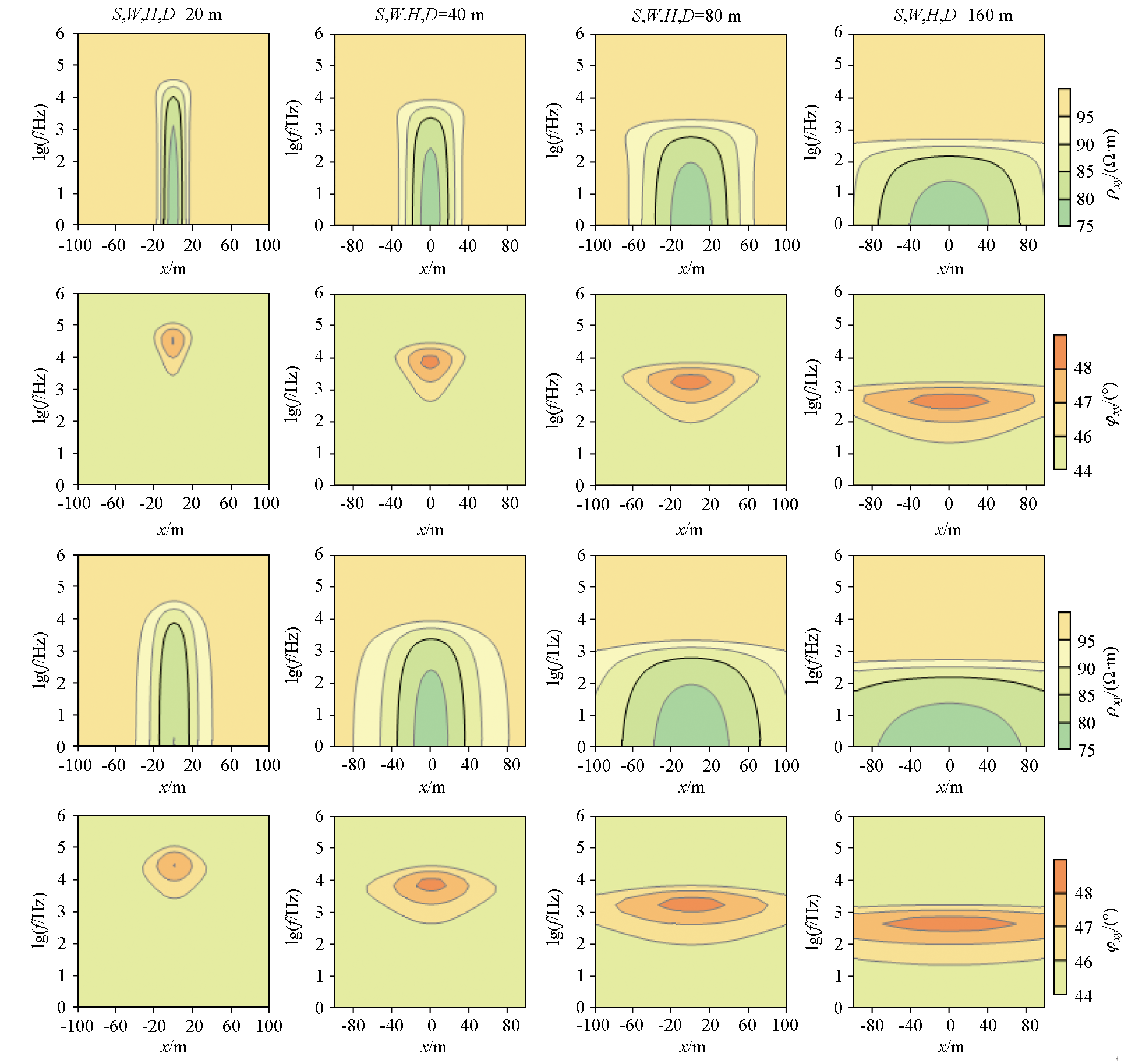
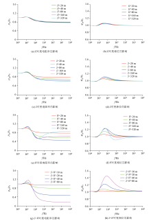
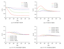
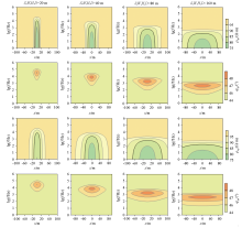
Abstract This study conducted the forward modeling of a 3D good conductor model under a uniform half-space background to investigate its response characteristics in a plane electromagnetic wave survey. The electromagnetic anomalies of a three-dimensional good conductor are primarily caused by the secondary field generated by static charge accumulated at interfaces. Consequently, higher relative resistivity differences between the target conductor and the surrounding rock correspond to greater response anomalies. Additionally, a smaller distance between observation electrodes and the target conductor is associated with greater relative response anomalies. Changes in the horizontal and vertical dimensions of a conductor pose different impacts of anomalies. Specifically, variations in vertical thickness have minor impacts on the anomalies. When a conductor has similar dimensions in the horizontal direction, its apparent resistivity response curve resembles a two-layer D-type sounding curve, with the relative anomalies intensifying as the horizontal sizes increase. However, in the case of significant differences between the two dimensions in the horizontal direction (with the larger dimension being at least eight times the smaller), the response curves observed in the directions of the larger and smaller dimensions differ. Notably, the apparent resistivity response curve observed in the direction of the larger dimension resembles a three-layer H-shaped sounding pattern characterized by high, low, and high values sequentially. In addition, the relative anomalies of apparent resistivity are generally more than two times those of phase, with apparent resistivity anomalies following the static effect law in the vertical direction. Specifically, apparent resistivity anomalies in high frequencies tend to extend to low frequencies, creating favorable conditions for anomaly identification. Therefore, apparent resistivity anomalies are more conducive to anomaly identification for good conductors.
|
|
Received: 26 June 2024
Published: 07 August 2025
|
|
|
|
|
|
|
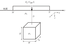
Simplified model
|

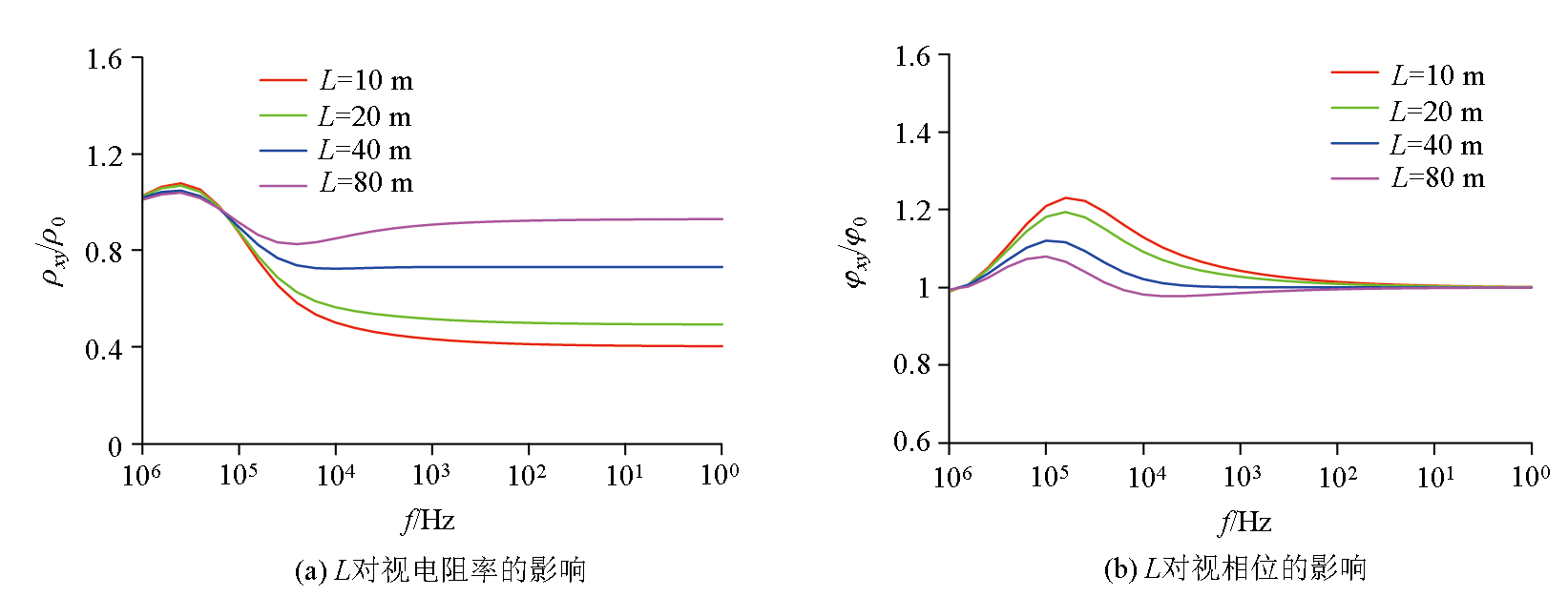
| 参数 | S/m | W/m | H/m | D/m | L/m | ρ1/(Ω·m) | ρ0/(Ω·m) | Max(${\delta }_{{\rho }_{xy}}$)/% | Max(${\delta }_{{\phi }_{xy}}$)/% | | L变化 | 20 | 20 | 20 | 10 | 10 | 10 | 100 | 60 | 23 | | 20 | 20 | 20 | 10 | 20 | 10 | 100 | 50 | 19 | | 20 | 20 | 20 | 10 | 40 | 10 | 100 | 28 | 12 | | 20 | 20 | 20 | 10 | 80 | 10 | 100 | 17 | 8 |
|
Model parameters and the maximum anomaly (electrode distance varies)
|
|
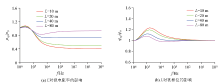
Normalized responses of the center point right above the target when electrode distance varies
|
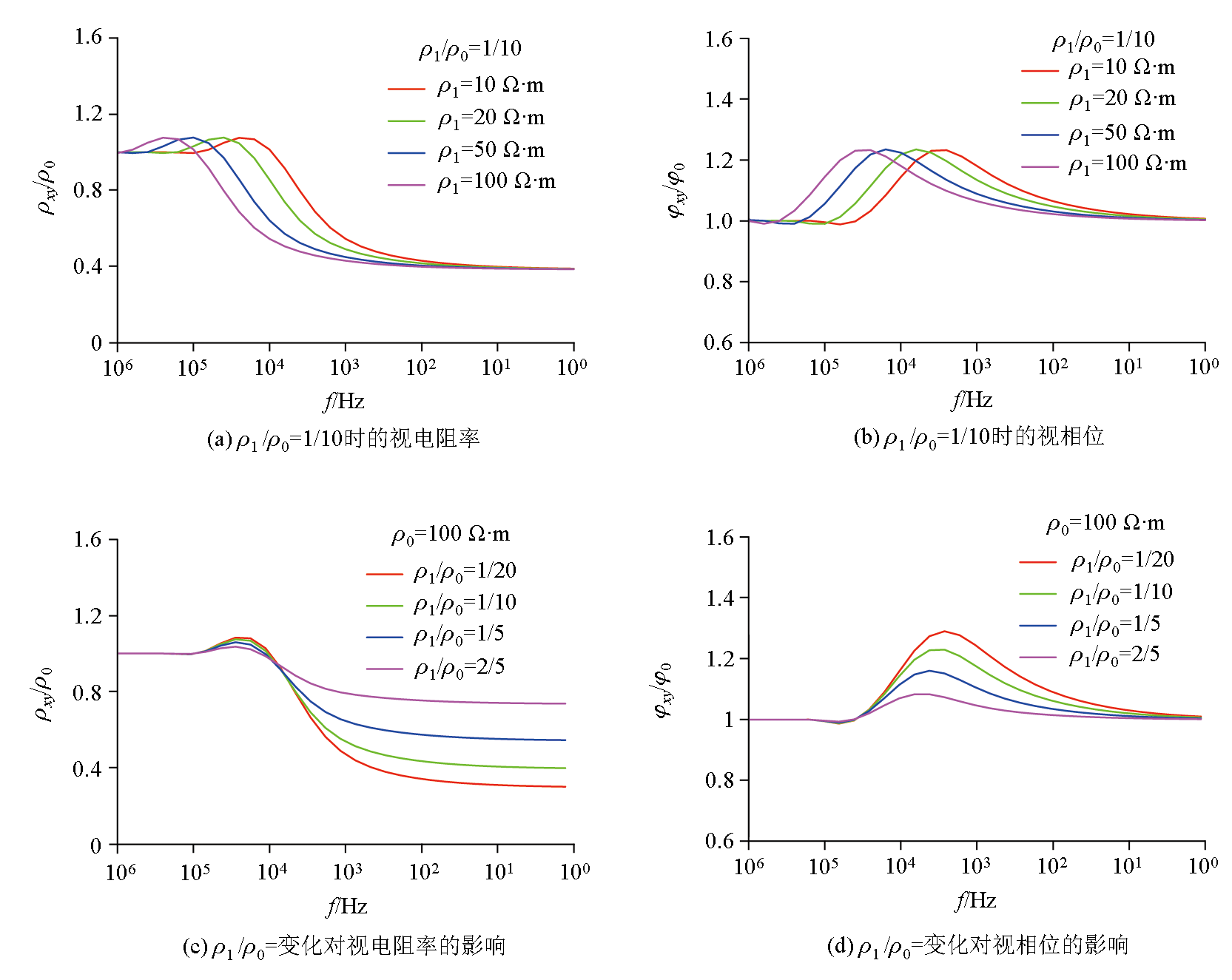
| 参数 | S/m | W/m | H/m | D/m | L/m | ρ1/(Ω·m) | ρ0/(Ω·m) | Max(${\delta }_{{\rho }_{xy}}$)/% | Max(${\delta }_{{\phi }_{xy}}$)/% | | ρ1/ρ0=1/10 | 80 | 80 | 80 | 40 | 20 | 10 | 100 | 61 | 23 | | 80 | 80 | 80 | 40 | 20 | 20 | 200 | 61 | 23 | | 80 | 80 | 80 | 40 | 20 | 50 | 500 | 61 | 23 | | 80 | 80 | 80 | 40 | 20 | 100 | 1000 | 61 | 23 | | ρ1/ρ0变化 | 80 | 80 | 80 | 40 | 20 | 5 | 100 | 71 | 29 | | 80 | 80 | 80 | 40 | 20 | 10 | 100 | 61 | 23 | | 80 | 80 | 80 | 40 | 20 | 20 | 100 | 46 | 16 | | 80 | 80 | 80 | 40 | 20 | 40 | 100 | 27 | 8 |
|
Model parameters and the maximum anomaly (resistivity varies)
|
|
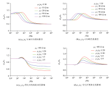
Normalized responses of the center point right above the target when resistivity varies
|
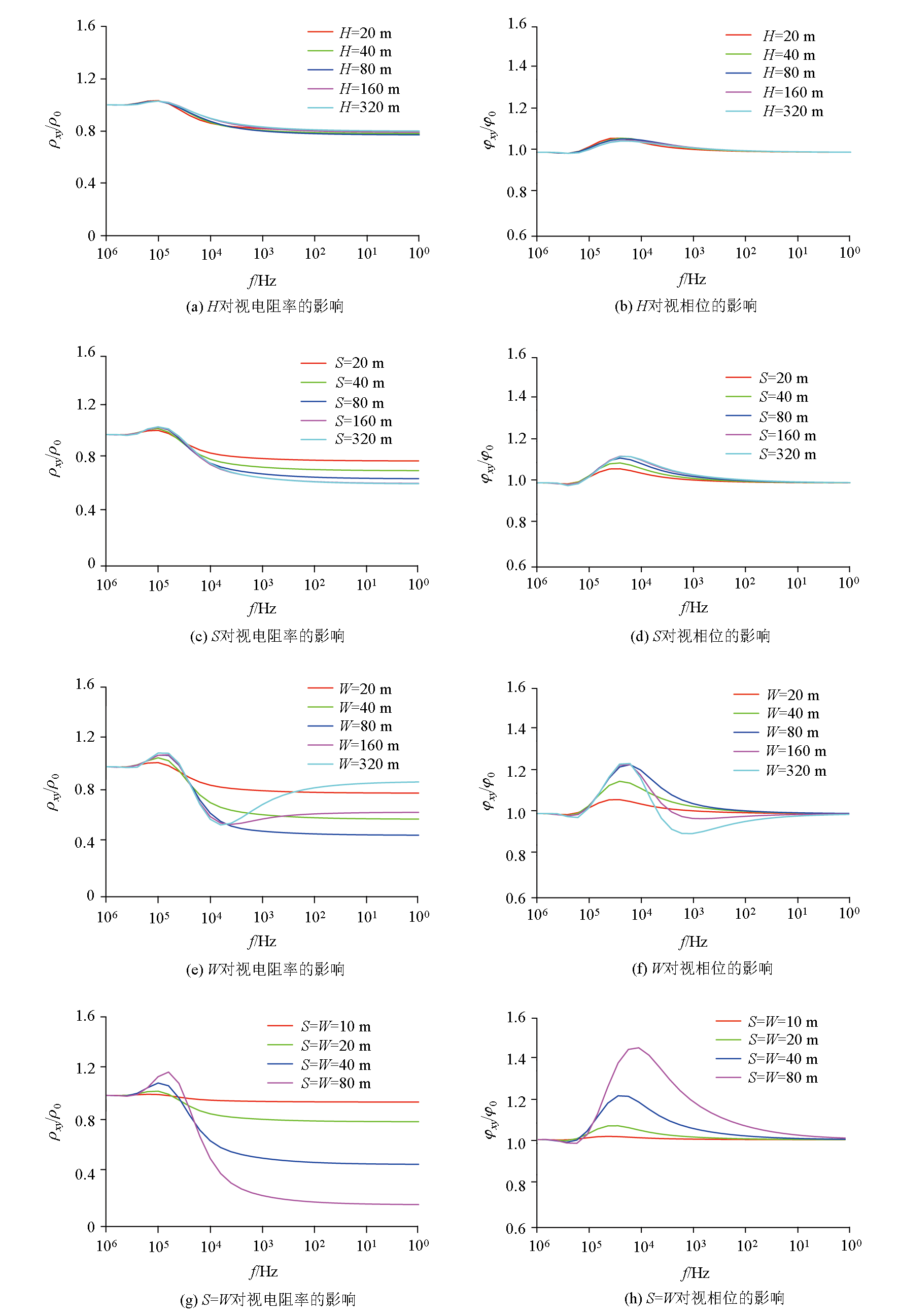
| 参数 | S/m | W/m | H/m | D/m | L/m | ρ1/(Ω·m) | ρ0/(Ω·m) | Max(${\delta }_{{\rho }_{xy}}$)/% | Max(${\delta }_{{\phi }_{xy}}$)/% | | H变化 | 80 | 80 | 20 | 80 | 20 | 10 | 100 | 15 | 5 | | 80 | 80 | 40 | 80 | 20 | 10 | 100 | 19 | 6 | | 80 | 80 | 80 | 80 | 20 | 10 | 100 | 23 | 7 | | 80 | 80 | 160 | 80 | 20 | 10 | 100 | 25 | 7 | | 80 | 80 | 320 | 80 | 20 | 10 | 100 | 25 | 7 | | S变化 | 20 | 20 | 20 | 20 | 20 | 10 | 100 | 20 | 7 | | 40 | 20 | 20 | 20 | 20 | 10 | 100 | 28 | 10 | | 80 | 20 | 20 | 20 | 20 | 10 | 100 | 34 | 12 | | 160 | 20 | 20 | 20 | 20 | 10 | 100 | 37 | 13 | | 320 | 20 | 20 | 20 | 20 | 10 | 100 | 37 | 13 | | W变化 | 20 | 20 | 20 | 20 | 20 | 10 | 100 | 20 | 7 | | 20 | 40 | 20 | 20 | 20 | 10 | 100 | 40 | 16 | | 20 | 80 | 20 | 20 | 20 | 10 | 100 | 52 | 24 | | 20 | 160 | 20 | 20 | 20 | 10 | 100 | 44 | 24 | | 20 | 320 | 20 | 20 | 20 | 10 | 100 | 44 | 24 | | S/W=1 | 10 | 10 | 20 | 20 | 20 | 10 | 100 | 5 | 2 | | 20 | 20 | 20 | 20 | 20 | 10 | 100 | 20 | 8 | | 40 | 40 | 20 | 20 | 20 | 10 | 100 | 53 | 21 | | 80 | 80 | 20 | 20 | 20 | 10 | 100 | 84 | 45 |
|
Model parameters and the maximum anomaly (target size varies)
|
|
Normalized responses of the center point right above the target when its size varies
|
|
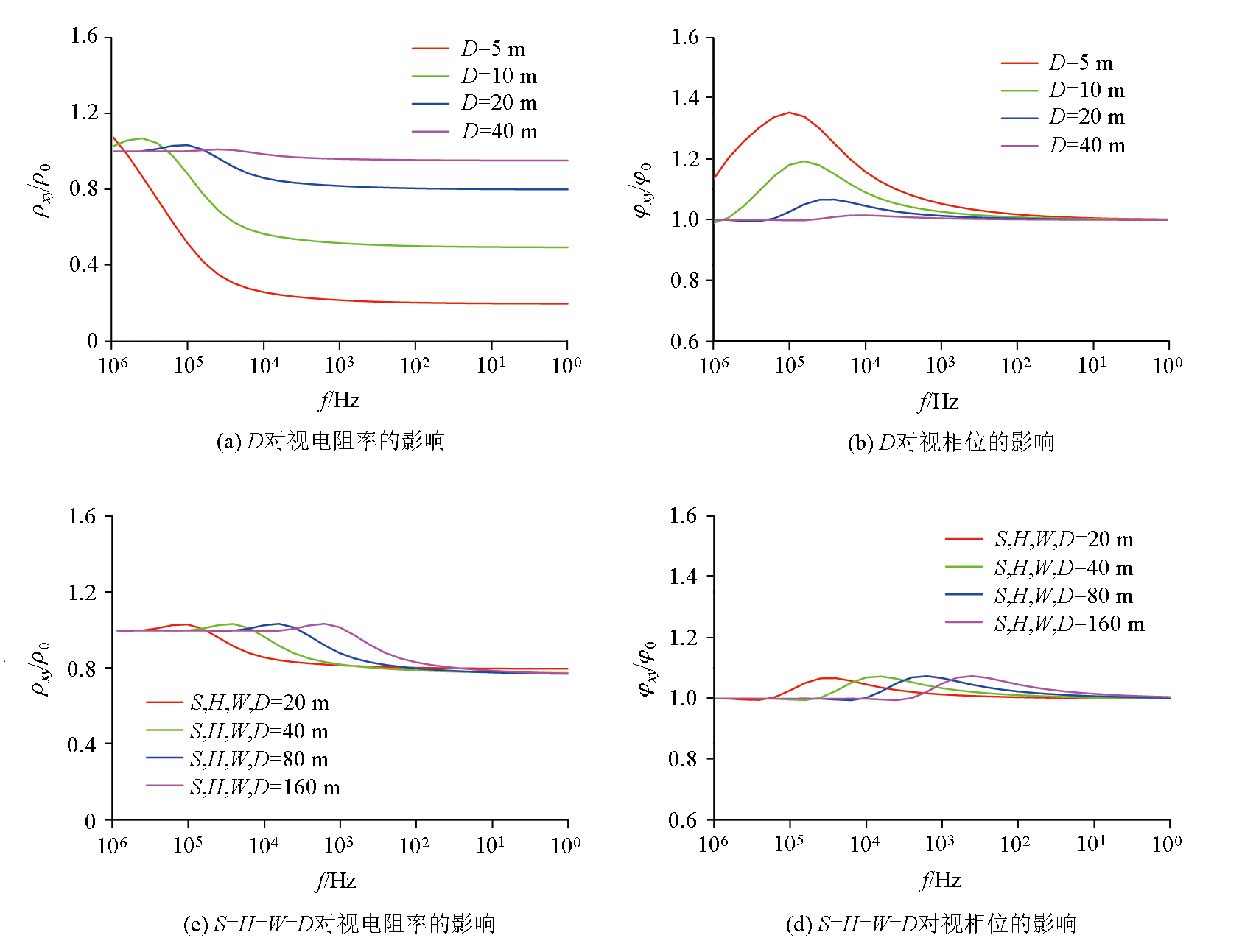
Normalized responses of the center point right above the target when its depth varies
|
| 参数 | S/m | W/m | H/m | D/m | L/m | ρ1/(Ω·m) | ρ0/(Ω·m) | Max(${\delta }_{{\rho }_{xy}}$)/% | Max(${\delta }_{{\phi }_{xy}}$)/% | | D变化 | 20 | 20 | 20 | 5 | 20 | 10 | 100 | 80 | 36 | | 20 | 20 | 20 | 10 | 20 | 10 | 100 | 51 | 19 | | 20 | 20 | 20 | 20 | 20 | 10 | 100 | 20 | 7 | | 20 | 20 | 20 | 40 | 20 | 10 | 100 | 5 | 2 | | S=W=H=D | 20 | 20 | 20 | 20 | 20 | 10 | 100 | 20 | 7 | | 40 | 40 | 40 | 40 | 20 | 10 | 100 | 22 | 7 | | 80 | 80 | 80 | 80 | 20 | 10 | 100 | 23 | 7 | | 160 | 160 | 160 | 160 | 20 | 10 | 100 | 23 | 7 |
|
Model parameters and the maximum anomaly (depth varies)
|
|
Profile response of cuboidal target
|
| [1] |
陈乐寿, 王光锷. 大地电磁测深法[M]. 北京: 地质出版社,1990.
|
| [1] |
Chen L S, Wang G E. Magnetotelluric sounding method[M]. Beijing: Geological Publishing House,1990.
|
| [2] |
李金铭. 地电场与电法勘探[M]. 北京: 地质出版社, 2005.
|
| [2] |
Li J M. Geoelectric field and electrical exploration[M]. Beijing: Geological Publishing House, 2005.
|
| [3] |
Kaufman A A, Keller G V. The magnetotelluric sounding method,method in geochemistry and geophysics[M]. Berlin: Springer, 2020. Amsterdam: Elsevisr Scientific,1981.
|
| [4] |
汤井田, 任政勇, 周聪, 等. 浅部频率域电磁勘探方法综述[J]. 地球物理学报, 2015, 58(8):2681-2705.
|
| [4] |
Tang J T, Ren Z Y, Zhou C, et al. Frequency-domain electromagnetic methods for exploration of the shallow subsurface:A review[J]. Chinese Journal of Geophysics, 2015, 58(8):2681-2705.
|
| [5] |
Lei D, Fayemi B, Yang L Y, et al. The non-static effect of near-surface inhomogeneity on CSAMT data[J]. Journal of Applied Geophysics, 2017,139:306-315.
|
| [6] |
Li J, Zhang X, Tang J T. Noise suppression for magnetotelluric using variational mode decomposition and detrended fluctuation analysis[J]. Journal of Applied Geophysics, 2020,180:104127.
|
| [7] |
伍亮, 李桐林, 朱成, 等. 大地电磁测深法中静态效应及其反演[J]. 地球物理学进展, 2015, 30(2):840-846.
|
| [7] |
Wu L, Li T L, Zhu C, et al. Research and inversion static effect in magnetotelluric[J]. Progress in Geophysics, 2015, 30(2):840-846.
|
| [8] |
李国瑞, 席振铢, 龙霞. 基于实测积累电荷静电场消除静态效应的方法[J]. 物探与化探, 2017, 41(4):730-735.
|
| [8] |
Li G R, Xi Z Z, Long X. Static displacement correction for frequency domain electromagnetic method based on second electrostatic field[J]. Geophysical and Geochemical Exploration, 2017, 41(4):730-735.
|
| [9] |
刘桂梅, 马为, 刘俊昌, 等. 大地电磁测深静态效应空间域拓扑处理技术研究[J]. 物探与化探, 2018, 42(1):118-126.
|
| [9] |
Liu G M, Ma W, Liu J C, et al. Spatial domain topological processing technique for studying static effect in magnetotelluric sounding[J]. Geophysical and Geochemical Exploration, 2018, 42(1):118-126.
|
| [10] |
杨天春, 胡峰铭, 于熙, 等. 天然电场选频法的响应特性分析与应用[J]. 物探与化探, 2023, 47(4):1010-1017.
|
| [10] |
Yang T C, Hu F M, Yu X, et al. Analysis and application of the responses of the frequency selection method of telluric electricity field[J]. Geophysical and Geochemical Exploration, 2023, 47(4):1010-1017.
|
| [11] |
Roy K K. Natural electromagnetic fields in pure and applied geophysics[M]. Cham: Springer Cham.
|
| [12] |
Vozoff K. Electromagnetic methods in applied geophysics[J]. Geophysical Surveys, 1980, 4(1):9-29.
|
| [13] |
Jiracek G R. Near-surface and topographic distortions in electromagnetic induction[J]. Surveys in Geophysics, 1990, 11(2):163-203.
|
| [14] |
Eikon Technologies Ltd.EMIGMA_full_manual.version 11.11.0,2024[K].https://www.petroseikon.com/EMIGMA/77ps/mt.php.

|
| [15] |
Wannamaker P E, Hohmann G W, SanFilipo W A. Electromagnetic modeling of three-dimensional bodies in layered earths using integral equations[J]. Geophysics, 1984, 49(1):60-74.
|
| [16] |
Ting S C, Hohmann G W. Integral equation modeling of three-dimensional magnetotelluric response[J]. Geophysics, 1981, 46(2):182-197.
|
| [17] |
任政勇, 陈超健, 汤井田, 等. 一种新的三维大地电磁积分方程正演方法[J]. 地球物理学报, 2017, 60(11):4506-4515.
|
| [17] |
Ren Z Y, Chen C J, Tang J T, et al. A new integral equation approach for 3D magnetotelluric modeling[J]. Chinese Journal of Geophysics, 2017, 60(11):4506-4515.
|
| [1] |
LUO Jiao, GUO Wen-Bo, LIU Chang-Sheng, ZHANG Ji-Feng, WANG Wei, XU Yi, ZHANG Xin-Xin, CHEN Jing. Definition of global apparent resistivity based on three components of the magnetic field for the interpretation of the ground-airborne frequency-domain electromagnetic data[J]. Geophysical and Geochemical Exploration, 2025, 49(3): 679-686. |
| [2] |
LI Dong, ZHANG Ming-Cai, WU Yuan-Yang. Exploring a correction technology for ground resistance in audio-frequency magnetotelluric measurements[J]. Geophysical and Geochemical Exploration, 2025, 49(3): 614-619. |
|
|
|
|