

0 引言
自然电位法是一种历史悠久的被动源探测方法,通常引起地表或者海底局部自然电位异常的源大致分为4类:地下水流动产生的流动电势、金属离子浓度差异引起的扩散电势、温度差异相关的温电效应产生的电势、与金属矿体和垃圾渗漏相关的氧化还原反应产生的电势[1]。近年来,自然电位法作为一种被动源探测方法在水文地质以及矿产勘查中发挥了重要作用。
1830年,Fox[2]就将自然电位法用于陆上的硫化物矿床调查。和陆上一样,海底多金属硫化物矿体上下部分发生氧化还原反应也会引起局部自然电位异常,20世纪70年代首次利用自然电位法进行海底多金属硫化物勘探[3]。由于海洋中人为的电磁噪声比陆地上少,因此利用电场传感器来探测海洋环境中的热液矿床非常有效[2]。近年来,海洋自然电位法被俄罗斯、日本、德国、中国等诸多国家用来寻找多金属硫化物。为了获得海底矿床的空间分布,需要对采集的自然电位数据进行反演。Patella[4]提出了概率密度成像法,获得了地下引起自然电位异常的源的位置,但该方法仅适用于单极电荷聚集的情况,像多金属硫化物矿体这种由氧化还原反应引起的自然电位异常,通常形成的是偶极源[5]。因此,Revil等[6]将概率密度成像拓展到偶极源情况。Kawada等[7]利用概率密度法获得了冲绳海槽lzena热液区可能存在电偶极子源。Biswas等[8]提出了模拟退火算法,用于复杂厚板状模型的自然电场数据的解释。基于有限元法的正演模拟,朱肖雄等[9]利用最小二乘正则化对自然电场场源进行了反演。Jardani等[1]通过对自然电位数据进行3D反演,获得了源电流密度的分布,进而确定地下流体的流动状态。Mendonca[10]使用格林公式来简化地电模型,同时考虑了围岩电导率、氧化还原电位梯度以及矿体的电导率对自然电位信号的影响,最后通过电荷守恒约束反演获得了源电流密度分布,并在秘鲁金矿的探测中进行了成功应用。Miller等[11]利用SimPEG开发的自然电位模块,3D反演获得了新西兰汤加里罗火山下的气、液分布,同时在模型中施加了范数约束。王文义[12]利用有限差分法实现了3D自然电位反演,并且在西南部印度洋脊玉皇热液区进行了应用。Guo等[13]利用自然电位法和直流电阻率法重建了大坝渗漏路径。
目前,自然电位法广泛用于硫化物矿体识别以及平面圈定中。为了利用自然电位数据反演获得矿体的空间结构,本文首先利用有限体积法离散了自然电位控制方程,通过数值解与解析解对比,验证了正演算法的可靠性;在反演算法中,将最小支撑约束与深度加权加入目标泛函中,通过对理论模型以及沙箱实验数据的反演验证了反演算法的可靠性。
1 3D自然电位正演模拟
1.1 自然电位控制方程
海底源电流密度
其中:
其中:
其中:
其中:
1.2 PARDISO 直接求解器的安装与求解
通常地球物理正演的控制方程可以简单表示为
表1 直接求解器与迭代求解器运行速度对比
Table 1
| 模型尺寸 | 运算时间/s | ||
|---|---|---|---|
| 最小二乘 迭代求解器 | 共轭梯度 迭代求解器 | PARDISO 直接求解器 | |
| 20 × 20 × 20 | 0.15 | 0.04 | 0.005 |
| 40 × 40 × 40 | 1.23 | 0.15 | 0.04 |
| 60 × 60 × 60 | 5.80 | 0.89 | 0.25 |
1.3 数值解与解析解对比
为了验证正演算法的可靠性,我们设计了一个100 × 100 ×100的3D网格(图 1a),整个空间为均匀电导率分布(1 S/m)。首先对均匀空间进行剖分,设置核心网格以及逐渐增大的不均匀网格来模拟无穷远,其中核心网格数目为74 ×74 ×74=405 224个,网格体积为1 m×1 m×1 m。设置Dirichlet边界条件,边界电势
图1
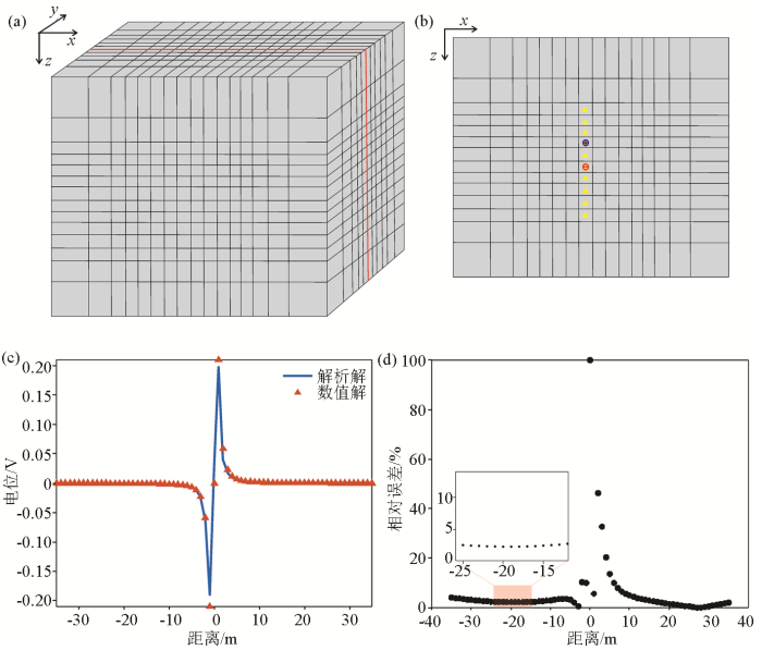
图1
有限体积法的正演响应与解析解对比
a—网格剖分示意;b—y=0 m切片(2D网格);c—数值解与解析解;d—相对误差
Fig.1
Comparison of forward response of finite volume method and analytic solutions
a—schematic diagram of mesh; b—the slice at y = 0 m (2D mesh); c—numerical and analytical solutions; d—relative error
1.4 海底多金属硫化物的自然电位响应特征
为了获得海底硫化物矿体的3D响应特征,建立如图 2a所示的模型。首先将地下介质剖分为40 × 40 × 30的网格,核心区域中网格的体积为20 m× 20 m × 10 m,用边界设置间距越来越大的变网格来模拟无穷远,x和y方向剖分范围为-214~214 m,z方向为-164~164 m,深度方向z = -100 m处为海底分界面(图 2c中的白色虚线位置),观测面距离海底10 m(深度方向z=-100 m),观测点数为13×13=169个(图 2a中的白色三角形为采样点)。模型空间中上半部分海水的电导率设置为3.2 S/m,海底以下围岩的电导率均为0.1 S/m。在海底以下空间中存在两个聚集着负电荷的长方体多金属硫化物块体,两个异常体的大小及体积一样,但是深度不一致。异常体在x方向的范围分别是-100 ~-40 m、40~140 m,在y方向的范围均为-30~30 m,z方向的深度范围分别是-80~-10 m、-60~20 m。两个多金属硫化物块体等效的电流密度均为1×10⁻³ A/m3,即每个小立方体的电流均为-1 A。
图2
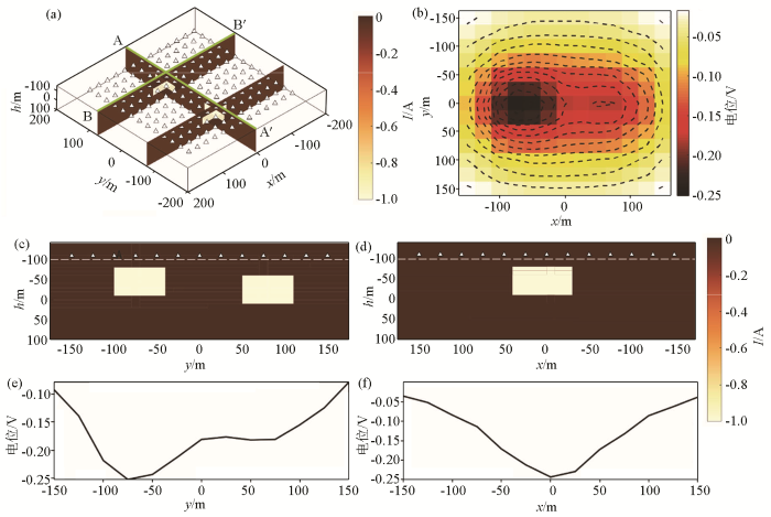
图2
3D正演模型及自然电位响应结果
a—模型及切片位置;b—接收器采集到的平面电场分布;c—剖面AA’是位于x = 0 m的切片;d—剖面BB’是位于y = -75 m的切片;e—测线AA’上的自然电位分布;f—测线BB’上的自然电位分布
Fig.2
3D model and forward response results
a—model and slice position; b—plane electric field distribution collected by receiver; c—section AA' is the slice at x = 0 m; d—BB' Slices are slices located at y = -75 m; e—spontaneous potential distribution on line AA'; f—spontaneous potential distribution on line BB'
2 3D自然电位反演方法
2.1 聚焦反演
其中:
通常2范数约束会使得反演得到的电流密度结构光滑,异常体的边界信息不够准确。因此,文中引入最小支撑稳定函数约束,使得反演结果在空间上更聚焦,更准确地反映海底硫化物空间分布。最小支撑稳定函数的定义如下[28]:
其中:
可以将上式简写为
其中:新的灵敏度矩阵
2.2 灵敏度矩阵计算
灵敏度矩阵为观测数据对模型的偏导数,通常反演中的灵敏度矩阵可以统一表示为[16]
由于自然电位反演是反演源的问题,所以矩阵
其中:矩阵
由于矩阵
其中:向量
3 合成模型
3.1 模型一
为了验证反演算法的可靠性,对图 2中3D模型的正演数据进行反演。反演中采用与正演相同的离散网格,设置迭代初始的正则化因子
3D反演结果如图 3所示。从反演得到的切片数据来看: 反演结果在平面上的分布与理论模型基本一致,同时异常体的位置反演的也比较准确,验证了聚焦反演在深度加权矩阵约束下能够较好地展示出深部异常体的电流密度分布情况。但相较于浅部异常体来说,深部异常体的下边界识别的不太清楚。同时由于聚焦反演的聚焦特性,反演得到的结果在体积上相对于理论模型会稍小一些。但反演得到的每个网格小立方体的电流最大值都达到了-1 A,和理论模型电流值较为吻合。
图3
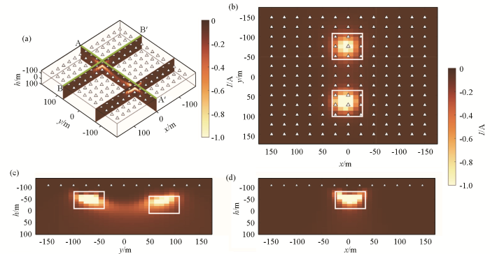
图3
3D自然电位反演结果及切片
a—反演结果及切片位置;b—位于z=0 m处的切面;c—剖面AA’的反演结果;d—剖面BB’的反演结果
Fig.3
3D self-potential inversion results and slices
a—inversion result and slice position; b—slice at z=0 m; c—inversion results of profile AA'; d—inversion of profile BB' performance result
3.2 模型二
图4
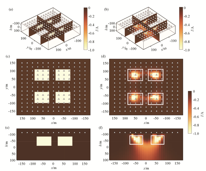
图4
3D自然电位模型及反演结果
a—模型;b—反演结果;c—模型切片(深度z=-65 m的切片);d—反演结果(深度z=-65 m处的切片);e—模型剖面(y=-65 m);f—反演结果(y=-65 m)
Fig.4
3D self-potential model and inversion results
a—inversion result and slice position; b—inversion result; c—model slice(at z=-65 m);d—inversion results of profile (slice at z = -65 m); e—model (y=-65 m); f—inversion result(y=-65 m)
3.3 模型三
图5
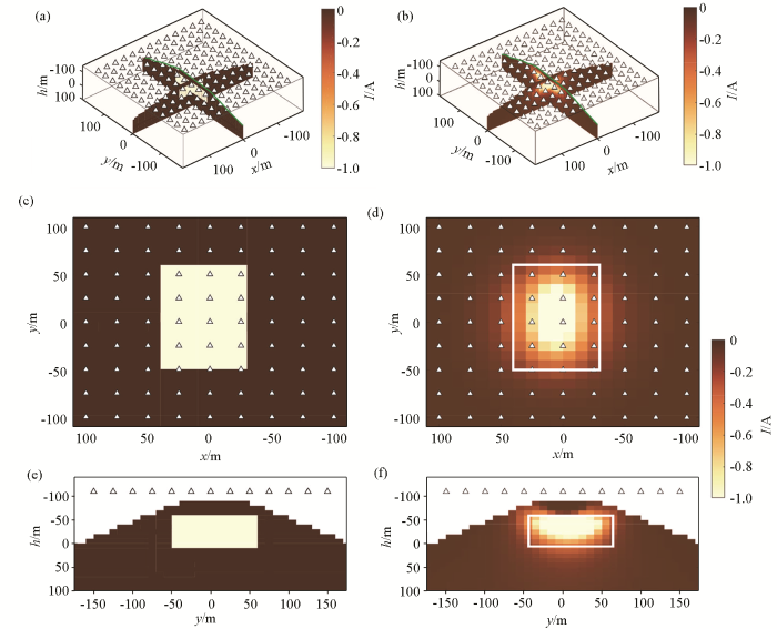
图5
起伏地形条件下的3D自然电位模型及反演结果
a—3D模型;b—反演结果;c—模型水平切片(z=-30m);d—反演结果水平切片(z=-30 m);e—模型垂直剖面(x = 0 m);f—反演结果剖面(x =0 m处)
Fig.5
3D self-potential model and inversion results
a—3D model; b—inversion result; c—horizontal slice of model (z=-30 m);d—horizontal slice was recovered by inversion (z=-30 m); e—vertical slice of model (x=0 m); f—vertical slice was recovered by inversion (slice at x=0 m)
图6
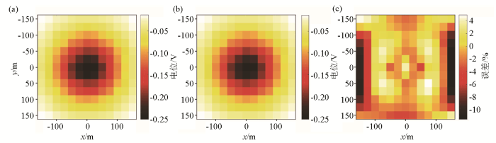
图6
正演的观测数据与预测数据
a—正演数据;b—反演得到的预测数据;c—正演数据与观测数据之间的误差
Fig.6
Observed data and predicted data obtained by inversion
a—observed data obtained by forward modeling; b—predicted data obtained from inversion; c—error between observed data and predicted data
4 沙箱实验
为了验证本文反演算法在实际中的应用效果,最后对实验室内开展沙箱实验获得的自然电位数据进行了反演。图 7所示的沙箱长0.9 m、宽0.45 m、高0.32 m。实验开始前,粒径相同的石英砂混合水溶液填满沙箱,模拟矿体附近的围岩,将金属棒埋在沙箱中间模拟硫化物矿体。实验过程中不断加水来控制潜水面的深度不变,确保氧化还原反应正常进行。实验中定期采集表面的2D自然电位数据以及矿体附近的3D自然电位数据、pH和Eh数据,观测氧化还原反应过程中引起的自然电位和化学数据变化。
图7
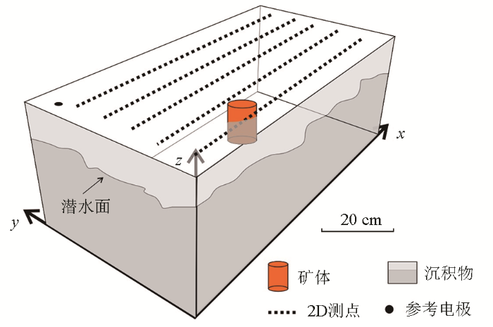
图8
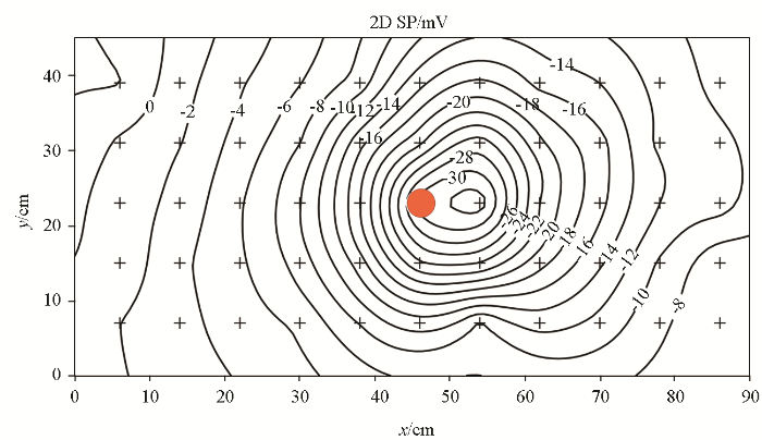
图8
氧化还原反应发生后的自然电位分布等值线
Fig.8
Contour diagram of self-potential distribution after the occurrence of redox reactions
图9
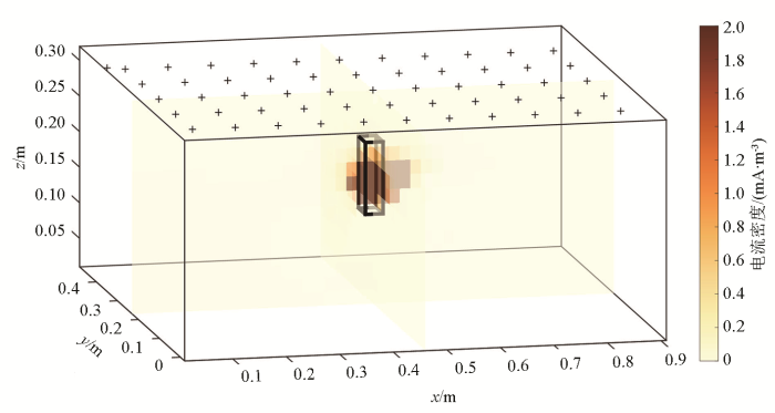
图10
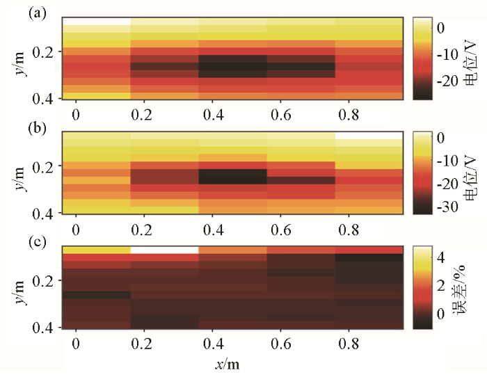
图10
沙箱试验的自然电位数据与反演的预测数据
a—沙箱试验数据;b—反演得到的预测数据;c—沙箱试验数据与观测数据之间的误差
Fig.10
self-potential data from sandbox experiment and predicted data obtained by inversion
a—sandbox experiment; b—predicted data obtained from inversion; c—error between experiment data and predicted data
5 结论
通过对合成模型和沙箱实验数据的自然电位3D正反演得到以下认识:①海底硫化物矿体通常会在近海底形成负的自然电位异常,且矿体越浅则异常越明显;②在合适的正则化因子、聚焦因子、深度加权矩阵等参数约束的条件下,自然电位3D聚焦反演能够较准确地得到海底空间多金属硫化物矿体的深度和边界范围等空间位置分布特征;③与迭代求解器相比,PARDISO直接求解器显著加快了3D反演计算效率。因此,本文提出的3D自然电位反演算法将会在未来硫化物资源勘探和评价中会发挥重要作用。
致谢
感谢中国石油大学(北京)朱忠民、王文义师兄在聚焦反演算法方面的指导,感谢法国萨瓦大学EDYTEM实验室André Revil教授提供沙箱实验的自然电位数据。衷心感谢评审专家对本文提出的修改意见。
参考文献
Three-dimensional inversion of self-potential data used to constrain the pattern of groundwater flow in geothermal fields
[J].
On the electro-magnetic properties of metalliferous veins in the mines of cornwall
[J].
DOI:10.1098/rstl.1830.0027
URL
[本文引用: 2]

In one of my communications to the Cornwall Geological Society on the high temperature of the interior of the earth, I ventured to express a belief that mineral veins, and the internal heat, are connected with electrical action. This opinion, founded as it was on the curious arrangement of the veins, &c. in primitive rocks, I have had the satisfaction to find confirmed by experiments made in some of the mines of Cornwall; and, I doubt not that the existence of electricity in metalliferous veins similarly circumstanced, and capable of conducting it, will prove to be as universal a fact, as the progressive increase of temperature under the earth’s surface is now admitted to be, much as my conclusions on this point were at one time controverted. In my first experiment I did not succeed in detecting any electricity; but in my second I had the gratification to observe considerable electrical action.
The self-potential method in geothermal exploration
[J].
DOI:10.1190/1.1440964
URL
[本文引用: 1]
Laboratory measurements and field data indicate that self‐potential anomalies comparable to those observed in many areas of geothermal activity may be generated by thermoelectric or electrokinetic coupling processes. A study using an analytical technique based on concepts of irreversible thermodynamics indicates that, for a simple spherical source model, potentials generated by electrokinetic coupling may be of greater amplitude than those developed by thermoelectric coupling. Before more quantitative interpretations of potentials generated by geothermal activity can be made, analytical solutions for more realistic geometries must be developed, and values of in‐situ coupling coefficients must be obtained. If the measuring electrodes are not watered, and if telluric currents and changes in electrode polarization are monitored and corrections made for their effects, most self‐potential measurements are reproducible within about ±5 mV. Reproducible short‐wavelength geologic noise of as much as ±10 mV, primarily caused by variation in soil properties, is common in arid areas, with lower values in areas of uniform, moist soil. Because self‐potential variations may be produced by conductive mineral deposits, stray currents from cultural activity, and changes in geologic or geochemical conditions, self‐potential data must be analyzed carefully before a geothermal origin is assigned to observed anomalies. Self‐potential surveys conducted in a variety of geothermal areas show anomalies ranging from about 50 mV to over 2 V in amplitude over distances of about 100 m to 10 km. The polarity and waveform of the observed anomalies vary, with positive, negative, bipolar, and multipolar anomalies having been reported from different areas. Steep potential gradients often are seen over faults which are thought to act as conduits for thermal fluids. In some areas, anomalies several kilometers wide correlate with regions of known elevated thermal gradient or heat flow.
Self-potential global tomography including topographic effects
[J].
DOI:10.1046/j.1365-2478.1997.570296.x
URL
[本文引用: 1]
This paper is an extension of a previous study, in which the principles of self‐potential ground surface tomography were outlined. The new arguments which are here set forth are the proper accounting for the topographic effects and a robust approach to global 3D tomography. The 2D case is initially considered in order to facilitate a full understanding of the new method. In order to gauge the topographic distortions, the concepts of slope effect and surface regularization are introduced, as suitable means to compute point by point correction factors of the measured self‐potential data, prior to the recognition of the tomographic images of the primary and induced electric sources underground. The tomographic approach is then developed by introducing again the concepts of the scanning function and of the charge occurrence probability function, which were amply dealt with in the previous paper. The new approach to 3D global tomography means here the composition of charge occurrence probability functions related to any two orthogonal surface components of the natural electric field, in order to account fully for the total surface component of the self‐potential field and hence to elicit the greatest amount of information. Two field examples are presented to show the full effectiveness of the proposed method. They refer, respectively, to a near‐surface investigation for archaeological purposes and to a very deep investigation in an active volcanic area.
金属矿自然电位的空间分布及其应用
[J].
Spatial distribution of spontaneous potential of metallic orebody and its application
[J].
Tomography of self-potential anomalies of electrochemical nature
[J].
DOI:10.1029/2001GL013631
URL
[本文引用: 1]
Ore deposits and buried metals like pipelines behave as dipolar electrical geobatteries in which the source is due to (1) variation of the redox potential with depth, (2) oxido‐reduction reactions acting at the ore body/groundwater contact, and (3) migration of electrons in the ore body itself between the reducing and oxidizing zones. This polarization mechanism is responsible for an electrical field at the ground surface, the so‐called self‐potential anomaly. A new quick‐look tomographic algorithm is developed to locate electrical dipolar sources in the subsurface of the Earth from the analysis of these self‐potential signals. We applied this model to the self‐potential anomaly discussed by Stoll et al. [1995] in the vicinity of the KTB‐boreholes drilled during the Continental Deep Drilling Project in Germany. The source of this self‐potential signal is related to the presence of massive graphite veins associated with steeply inclined fault zones within the gneisses and observed in the KTB‐boreholes.
Self-potential mapping using an autonomous underwater vehicle for the Sunrise deposit,Izu-Ogasawara arc,southern Japan
[J].DOI:10.1186/s40623-018-0913-6 [本文引用: 1]
Interpretation of self-potential anomaly over 2-D inclined thick sheet structures and analysis of uncertainty using very fast simulated annealing global optimization
[J].DOI:10.1007/s40328-016-0176-2 URL [本文引用: 1]
基于最小二乘正则化的自然电场场源反演成像
[J].
Inversion for self-potential sources based on the least squares regularization
[J].
Forward and inverse self-potential modeling in mineral exploration
[J].
Distribution of vapor and condensate in a hydrothermal system:Insights from self-potential inversion at mount Tongariro,new zealand
[J].
DOI:10.1029/2018GL078780
URL
[本文引用: 1]
Inversion of self‐potential data for source current density, js, in complex volcanic settings, yields hydrological information without the need for a prior groundwater flow model; js contains information about pH, pore saturation, and permeability, from which we infer the distribution of liquid and vapor phases. To understand the hydrothermal flow dynamics and hydraulic connectivity between surface thermal features at Mount Tongariro volcano, New Zealand, we undertook a reconnaissance scale self‐potential survey and developed an inversion routine for js, constrained by an existing 3‐D conductivity model from magnetotelluric measurements. The 3‐D distribution of js at Mount Tongariro reveals a discontinuous zero js zone interpreted as vapor or residually saturated pore space, surrounded by low to moderate js interpreted as circulating condensate liquid. Bounding faults act as conduits for down flowing groundwater or condensate, as well as barriers for the hydrothermal system. Localized small‐scale circulation associated with individual surface thermal features, rather than a single circulating system, accounts for the lack of widespread anomalous geochemical observations prior to the 2012 Te Maari eruption.
Seepage detection in earth-filled dam from self-potential and electrical resistivity tomography
[J].DOI:10.1016/j.enggeo.2022.106750 URL [本文引用: 1]
Self-potential signals generated by the corrosion of buried metallic objects with application to contaminant plumes
[J].
Pixels and their neighbors:Finite volume
[J].
DOI:10.1190/tle35080703.1
URL
[本文引用: 1]
We take you on the journey from continuous equations to their discrete matrix representations using the finite-volume method for the direct current (DC) resistivity problem. These techniques are widely applicable across geophysical simulation types and have their parallels in finite element and finite difference. We show derivations visually, as you would on a whiteboard, and have provided an accompanying notebook at http://github.com/seg to explore the numerical results using SimPEG ( Cockett et al., 2015 ).
Evaluation of parallel direct sparse linear solvers in electromagnetic geophysical problems
[J].DOI:10.1016/j.cageo.2016.01.009 URL [本文引用: 1]
Two-level dynamic scheduling in PARDISO:Improved scalability on shared memory multiprocessing systems
[J].DOI:10.1016/S0167-8191(01)00135-1 URL [本文引用: 1]
Large-scale sparse inverse covariance matrix estimation
[J].
3D magnetic inversion with data compression and image focusing
[J].
DOI:10.1190/1.1512749
URL
[本文引用: 1]
We develop a method of 3‐D magnetic anomaly inversion based on traditional Tikhonov regularization theory. We use a minimum support stabilizing functional to generate a sharp, focused inverse image. An iterative inversion process is constructed in the space of weighted model parameters that accelerates the convergence and robustness of the method. The weighting functions are selected based on sensitivity analysis. To speed up the computations and to decrease the size of memory required, we use a compression technique based on cubic interpolation.
von Matt U.Generalized cross-validation for large-scale problems
[J].
Induced polarization response of porous media with metallic particles—Part 3:A new approach to time-domain induced polarization tomography
[J].
Geophysical inverse theory and regularization problems
[M].
3D inversion of magnetic data
[J].
DOI:10.1190/1.1443968
URL
[本文引用: 1]
We present a method for inverting surface magnetic data to recover 3-D susceptibility models. To allow the maximum flexibility for the model to represent geologically realistic structures, we discretize the 3-D model region into a set of rectangular cells, each having a constant susceptibility. The number of cells is generally far greater than the number of the data available, and thus we solve an underdetermined problem. Solutions are obtained by minimizing a global objective function composed of the model objective function and data misfit. The algorithm can incorporate a priori information into the model objective function by using one or more appropriate weighting functions. The model for inversion can be either susceptibility or its logarithm. If susceptibility is chosen, a positivity constraint is imposed to reduce the nonuniqueness and to maintain physical realizability. Our algorithm assumes that there is no remanent magnetization and that the magnetic data are produced by induced magnetization only. All minimizations are carried out with a subspace approach where only a small number of search vectors is used at each iteration. This obviates the need to solve a large system of equations directly, and hence earth models with many cells can be solved on a deskside workstation. The algorithm is tested on synthetic examples and on a field data set.
Minimum support nonlinear parametrization in the solution of a 3D magnetotelluric inverse problem
[J].DOI:10.1088/0266-5611/20/3/017 URL [本文引用: 1]
