基于监督下降法的大地电磁二维反演及应用研究

doi:10.11720/wtyht.2024.1417

基于监督下降法的大地电磁二维反演及应用研究

付兴^,, 谭捍东^,, 董岩, 汪茂

中国地质大学(北京) 地球物理与信息技术学院,北京 100083

Application of supervised descent method for 2D magnetotelluric inversion and its application

FU Xing^,, TAN Han-Dong^,, DONG Yan, WANG Mao

School of Geophysics and Information Technology, China University of Geosciences, Beijing 100083,China

通讯作者: 谭捍东(1966-),男,教授,地球探测与信息技术专业,主要从事电法勘探理论及应用研究工作。Email:thd@cugb.edu.cn

责任编辑: 王萌

收稿日期: 2023-10-13 修回日期: 2023-10-20

基金资助:

国家自然科学基金项目(41830429)
山西省重点研发计划项目(202102080301001)

Received: 2023-10-13 Revised: 2023-10-20

作者简介 About authors

付兴(1999-),男,硕士研究生,地球探测与信息技术专业,主要研究方向为机器学习与电法勘探算法。Email:2010210060@email.cugb.edu.cn

摘要

传统的大地电磁二维反演方法较为成熟,但仍存在反演结果依赖初始模型和正则化参数选取、容易陷入局部极小值等问题。监督下降法是一种学习平均下降方向来预测数据残差的机器学习算法。本文尝试采用监督下降法解决传统的大地电磁二维反演存在的问题,基于监督下降法理论开发了大地电磁二维反演算法,设计理论模型合成算例验证了算法的正确性,并对西藏高原实测数据进行反演,检验了监督下降法的实用性。理论模型合成数据和实测数据反演结果表明,相较于传统的非线性共轭梯度反演,基于监督下降法的反演具有收敛速度快、反演效果好、抗噪能力强等特点。

关键词： 大地电磁法; 二维反演; 机器学习; 监督下降法; 非线性共轭梯度反演

Abstract

Traditional two-dimensional inversion methods of magnetotelluric are mature, but there are still some problems, such as reliance on the initial model, reliance on regularization parameter selection, and easy to fall into local minimum. In order to solve the above problems, this paper adopts the supervised descent method to improve the effect of two-dimensional inversion of magnetotelluric. The supervised descent method is a machine learning algorithm that learns the average descending direction to predict the residual of data. Based on the theory of supervised descent method, this paper develops the two-dimensional inversion algorithm of magnetotelluric, designs the theoretical model synthesis example to verify the correctness of the algorithm, and inverts the measured data on the Tibet Plateau to test the practicability of the supervised descent method. The inversion results of the theoretical model synthesis data and the measured data show that, compared with the traditional nonlinear conjugate gradient inversion, the inversion based on the supervised descent method has the characteristics of fast convergence speed, good inversion effect, and strong anti-noise ability.

Keywords： magnetotelluric; 2D inversion; machine learning; supervised descent method; gradient Non-linear conjugate gradient

PDF (5394KB) 元数据多维度评价相关文章导出 EndNote| Ris| Bibtex 收藏本文

本文引用格式

付兴, 谭捍东, 董岩, 汪茂. 基于监督下降法的大地电磁二维反演及应用研究[J]. 物探与化探, 2024, 48(1): 175-184 doi:10.11720/wtyht.2024.1417

FU Xing, TAN Han-Dong, DONG Yan, WANG Mao. Application of supervised descent method for 2D magnetotelluric inversion and its application[J]. Geophysical and Geochemical Exploration, 2024, 48(1): 175-184 doi:10.11720/wtyht.2024.1417

0 引言

大地电磁测深法(MT)是一种通过观测天然交变电磁场来对地电构造进行研究的物探方法,大地电磁法的频域很宽,其探测深度距地表有几百米到数百公里不等,具有分辨率高,穿透能力强,勘探深度大以及效率高等实际优点,被广泛应用于金属矿产普查、勘探地热和油气田等领域^[1]。

大地电磁二维反演常采用高斯牛顿法^[2]、OCCAM法^[3]、非线性共轭梯度法^[4]等,这些方法在最小化目标函数时各有优劣,但都无法在迭代过程中避免雅可比矩阵或海森矩阵的计算,且存在陷入局部极小值的风险,导致反演效果变差。

近些年随着计算机行业的发展,机器学习成功在多种领域取得不错的效果^[5]。机器学习能够挖掘变量与标签之间的关联,并学习其关联进行预测,大大减少反演时间,提升计算效率^[6]。

监督下降法(SDM)在人脸识别技术中被广泛使用^[7-8],后被带入到多领域进行研究^[9⇓-11]。采取监督下降法解决地球物理勘探领域的问题也取得了不错的成效^[12],模型与正演响应合并构成的训练集在进行一维瞬变电磁(TEM)反演中发挥了重要的作用^[13]。监督下降法分为离线训练和在线预测两个阶段,在离线训练阶段,通过学习大量模型及其响应得出平均下降步长。在预测阶段,采用学习的步长进行迭代预测。平均步长具有较好的指导作用,避免了迭代陷入局部极小的风险,提升了反演的效果。此外,监督下降法并不需要计算雅可比矩阵和海森矩阵,避免了内存浪费的同时,提升了反演的效率。

本文采用监督下降法理论改进大地电磁二维数据反演算法,编写相关代码并设计理论模型验证算法的正确性,对其抗噪能力及实用性进行检验。相较于传统的非线性共轭梯度反演,基于监督下降法的反演具有收敛速度快、反演效果好、抗噪能力强等特点。

1 大地电磁二维正反演简介

1.1 大地电磁二维有限单元法正演

忽略位移电流和磁导率的影响,时间因子为e^-i^ωt,大地电磁场满足麦克斯韦方程组:

(1)

\begin{array}{l} \nabla \times E = i μ_{0} ω H, \\ \nabla \times H = σ E, \end{array}

式中:σ为介质的电导率;μ₀为介质的磁导率;E为电场强度;H为磁感应强度。由式(1)可推导出赫姆霍兹方程组:

(2)

\begin{array}{l} \nabla^{2} E - k^{2} E = 0, \\ \nabla^{2} H - k^{2} H = 0, \end{array}

式中:k为波数,k= $\sqrt[]{- i ω μ_{0} σ}$ ,大地电磁二维有限单元正演的变分问题为^[14]:

(3)

\{\begin{array}{l} G (u) = \int_{Ω}^{} [\frac{1}{2} τ {(\nabla u)}^{2} - \frac{1}{2} λ u^{2}] d Ω + \int_{C D}^{} \frac{1}{2} τ k u^{2} d Γ, \\ u_{A B} = 1, \\ δ G (u) = 0, \end{array}

式中:AB为上边界,CD为下边界。

(4)

\begin{array}{l} T E : u = E_{x}, τ = \frac{1}{i ω μ_{0}}, λ = σ, \\ T M : u = H_{x}, τ = \frac{1}{σ}, λ = i ω μ_{0}, \end{array}

对图1所有单元进行离散,式(3)变为:

(5)G

(u)

\sum_{Ω} \int_{ε}^{} \frac{1}{2}

{(\nabla u)}^{2}

dΩ-

\sum_{Ω} \int_{ε}^{} \frac{1}{2}

λu²dΩ+

\sum_{C D} \int_{ε}^{} \frac{1}{2}

τku²dΓ=

\frac{1}{2}

u^TKu,

式中:K为总体系数矩阵,求取式(5)的极值,可得

(6)Ku=0,

可得出各节点的u,相应的视电阻率及阻抗相位为:

(7)

\begin{array}{l} Z_{T E} = E_{x} / \frac{1}{i ω μ_{0}} \frac{\partial E_{x}}{\partial z}, \\ ρ_{s}^{T E} = \frac{1}{ω μ_{0}}| Z_{T E} |^{2}, φ_{T E} = a r c t a n (\frac{I M (Z_{T E})}{R E (Z_{T E})}), \\ Z_{T M} = - \frac{1}{σ} \frac{\partial H_{x}}{\partial z} / H_{x}, \\ ρ_{s}^{T M} = \frac{1}{ω μ_{0}}| Z_{T E} |^{2}, φ_{T M} = a r c t a n (\frac{I M (Z_{T M})}{R E (Z_{T M})}) 。 \end{array}

图1

新窗口打开| 下载原图ZIP| 生成PPT

图1 部分单元网格

Fig.1 Sketch of partial grid

1.2 大地电磁二维非线性共轭梯度反演

常规的大地电磁二维反演方法有高斯牛顿法、OCCAM法、非线性共轭梯度法。本文将采用非线性共轭梯度反演与基于监督下降法的反演进行对比,下面概要介绍非线性共轭梯度反演方法。

定义大地电磁二维反演目标函数如下^[15]:

(8)Φ(m)=

{(d}_{o b s} - F {(m))}^{T}

V^-1(d_obs-F(m))+λ

{(m}_{0} {- m)}^{T}

L^TL(m₀-m),

式中:m为模型参数;F(m)为求取阻抗张量的正演函数;d_obs为模型正演响应或实测数据;V为协方差矩阵;λ为正则化参数;L为二次差分拉普拉斯算子;m₀为先验信息,目标函数具有数据拟合差最小和模型最光滑的双重约束。

目标函数的梯度为:

(9)g=-2A^TV^-1e+2λL^TL

(m_{0} - m)

其中:A表示雅可比矩阵,数据误差向量:e=d_obs-F(m)。

非线性共轭梯度反演的具体步骤如下^[16-17]:

1)i=0时,设定初始模型m_i,计算梯度r_i=g_i;

2)取M_i= $‖r_{i}‖$ ,为预处理算子,共轭梯度方向u_i= $M_{i}^{- 1}$ r_i;

3)求解r_i=0,得出最优搜索步长α_i;

4)m_i₊₁=m_i+α_iu_i,r_i₊₁=g_i₊₁;

5)若r_i₊₁小于预设的最小值,则反演结束,否则令u_i₊₁= $M_{i + 1}^{- 1}$ r_i₊₁+ $β_{i + 1}^{T}$ u_i,其中β_i₊₁= $\frac{(r_{i + 1} M_{i + 1}^{- 1} r_{i + 1} - r_{i}^{T} M_{i}^{- 1} r_{i})}{r_{i}^{T} M_{i}^{- 1} r_{i}}$ ;

6)取i=i+1,回到步骤3),直至收敛,反演结束。

2 基于监督下降法的大地电磁二维反演

监督下降法运用机器学习理论,采取半监督学习方式,分为训练和预测两个阶段。训练阶段通过对训练集的学习,得到一组平均下降方向。预测阶段运用平均下降方向迭代计算数据残差,进而进行迭代。监督下降法的流程如图2。

图2

新窗口打开| 下载原图ZIP| 生成PPT

图2 监督下降流程

Fig.2 The flowchart of supervised descent method inversion

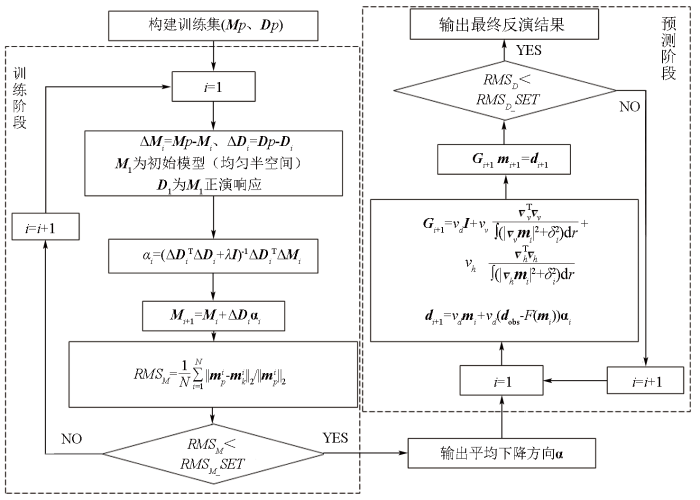
2.1 训练阶段

在进行大地电磁反演计算时,定义目标函数如下:

(10)Φ

(m)

{‖d_{o b s} - F (m)‖}_{2}^{2}

对式(10)的正演函数F(m)进行一阶Taylor展开,求取对m的极小值,可得:

(11)Δm=

(J^{T} {J)}^{- 1}

J^TΔ d,

其中:J为雅可比矩阵;Δm=m-m₁;Δd=d_obs-F(m);α= ${(J}^{T} {J)}^{- 1}$ J^T,α为迭代步长。由于正演数据存在非线性,常规反演通常采取不断迭代的方式来求取Φ(m)关于m的极小值,计算雅可比矩阵及海森矩阵是在进行常规反演时较为消耗计算时间和占用内存空间的一步。况且,上述目标函数在此时容易陷入局部极小,所以,需要大量的模型迭代来获得迭代最优方向。

此时,相较于每次迭代均需计算雅可比矩阵或海森矩阵且每步均需搜索下降步长的常规大地电磁反演,引入机器学习的思想,通过学习的平均下降方向,使目标函数快速趋于极小值的方法可以节约大量计算时间以及大量内存空间,同时避免目标函数陷入局部极小值。

合成一组训练集(标签集M_P和数据集D_P),为了计算下降方向,求下式极小值:

(12)Θ(m)=

{‖Δ M - Δ D \times α‖}_{F}^{2}

其中: ${‖\cdot‖}_{F}^{2}$ 为矩阵的F范数,ΔM以及ΔD的表达式如下:

(13)ΔM₁=M_p-M₁,M_p=

[\begin{array}{l} (m_{p}^{1})^{T} \\ (m_{p}^{2})^{T} \\ ︙ \\ (m_{p}^{N})^{T} \end{array}]

,M₁=

[\begin{array}{l} (m_{1})^{T} \\ (m_{1})^{T} \\ ︙ \\ (m_{1})^{T} \end{array}]

(14)ΔD₁=D_p-D₁,D_p=

[\begin{array}{l} F {(m_{p}^{1})}^{T} \\ F {(m_{p}^{2})}^{T} \\ ︙ \\ F {(m_{p}^{N})}^{T} \end{array}]

,D_p=

[\begin{array}{l} F {(m_{1})}^{T} \\ F {(m_{1})}^{T} \\ ︙ \\ F {(m_{1})}^{T} \end{array}]

其中:m₁为初始模型(通常为均匀半空间); $m_{p}^{n}$ 为输入的模型集中的第n个模型。采取最小二乘法求解上述方程的极小值,可得:

(15)α_i=

{(Δ {D_{i}}^{T} Δ D_{i} + λ I)}^{- 1}

{D_{i}}^{T}

ΔM_i,

式中:i为迭代次数;λ为阻尼系数(可与相加的内容呈现比例关系), ${M_{i}}_{+ 1}$ 表达式如下:

M_i₊₁=M_i+ΔD_iα_i, (16)

在此阶段,数据拟合差RMS_D与模型拟合差RMS_M为:

(17)RMS_D=

\frac{1}{N} \overset{N}{\sum_{i = 1}} \frac{{‖m_{p}^{i} - m_{k}^{i}‖}_{2}}{{‖m_{p}^{i}‖}_{2}}

,RMS_M=

\frac{1}{N} \overset{N}{\sum_{i = 1}} \frac{{‖F (m_{p}^{i}) - F (m_{k}^{i})‖}_{2}}{{‖F (m_{p}^{i})‖}_{2}}

当模型拟合差趋于稳定、足够小或者达到了预设的最大迭代次数时,训练阶段结束。

2.2 预测阶段

将上阶段的平均步长用于该阶段的计算,具体过程如下:

(18)m_i₊₁=m_i+

[d_{o b s} - F (m_{i})]

α_i,

从i=1开始计算,m₁与训练过程的初始模型相同。当F(m_i)与d_obs间的数据残差为0时,停止迭代,输出反演结果。

为解决反演的多解性问题,考虑在预测阶段加入吉洪诺夫正则化来解决这一问题。

(19)

Θ_{R}^{p r} (m_{i})

=Θ_d

(m_{i})

+υ_vΘ_v

(m_{i})

+υ_hΘ_h

(m_{i})

式(19)为进行正则化的目标函数,其中υ_v、υ_h为垂直方向以及水平方向的正则化系数。

(20)Θ_d

(m_{i})

=υ_d

{‖m_{i} - m_{i - 1} - [d_{o b s} - F (m_{i - 1})] α_{i - 1}‖}^{2}

Θ_v

(m_{i})

b_{v}^{2} \int_{D}^{} (| \nabla_{v} m_{i} |^{2} + δ_{i - 1}^{2})

drΘ_h(m_i)=

b_{h}^{2} \int_{D}^{}

\nabla_{h}

m_i|²+

δ_{i - 1}^{2}

)dr,

式中:

(21)$ \begin{array}{l} \boldsymbol{b}_{v}^{2}=\frac{1}{\int_{D}\left(\left|\nabla_{v} \boldsymbol{m}_{i-1}\right|^{2}+\boldsymbol{\delta}_{i-1}^{2}\right) \mathrm{d} r} \\ \boldsymbol{b}_{h}^{2}=\frac{1}{\int_{D}\left(\left|\nabla_{h} \boldsymbol{m}_{i-1}\right|^{2}+\boldsymbol{\delta}_{i-1}^{2}\right) \mathrm{d} r}, \\ \boldsymbol{\delta}_{i-1}^{2}=\frac{\left\|\boldsymbol{d}_{\text {obs }}-F\left(\boldsymbol{m}_{i-1}\right)\right\|^{2}}{\left\|\boldsymbol{d}_{\text {obs }}\right\|^{2}} \times \frac{1}{\boldsymbol{\Delta}} \end{array}$

式中:υ_d=1/ ${‖d_{o b s}‖}^{2}$ 为归一化参数;D为计算空间;$\boldsymbol{\nabla}_{v}$、$\boldsymbol{\nabla}_{h}$为垂直方向以及水平方向的差分算子; $\overset{\land}{Δ}$ 为与网格大小有关的超系数。

求取式(19)的极小值进行偏导处理,可得下式,化简后,可得

(22)G_im_i=d_i,

(23)$ \begin{array}{l} \boldsymbol{G}_{i}=v_{d} \boldsymbol{I}+v_{v} \frac{\boldsymbol{\nabla}_{v}^{\mathrm{T}} \boldsymbol{\nabla}_{v}}{\int_{D}\left(\left|\nabla_{v} \boldsymbol{m}_{i-1}\right|^{2}+\boldsymbol{\delta}_{i-1}^{2}\right) \mathrm{d} r} \\ +\frac{\boldsymbol{\nabla}_{h}^{\mathrm{T}} \boldsymbol{\nabla}_{h}}{\int_{D}\left(\left|\nabla_{h} \boldsymbol{m}_{i-1}\right|^{2}+\boldsymbol{\delta}_{i-1}^{2}\right) \mathrm{d} r} \\ \boldsymbol{d}_{i}=v_{d} \boldsymbol{m}_{i-1}+v_{d}\left(\boldsymbol{d}_{\mathrm{obs}}-F\left(\boldsymbol{m}_{i-1}\right)\right) \boldsymbol{\alpha}_{i-1} \end{array}$

求解式(22),解出的m_i,利用m_i进行下次迭代,直至数据拟合差停止变小或小于一定数值,数据拟合差公式如下:

(24)RMS_D=

\frac{{‖d_{o b s} - F (m_{i})‖}_{2}}{{‖d_{o b s}‖}_{2}}

最大训练次数的步长预测完后,得出的数据拟合差未达到标准或者预测结果未达到期望,采取重启步长算法,即从第一个步长开始,进行新一轮的预测,直至数据拟合差足够小或不再减少。

3 理论模型合成数据二维反演算例

大地电磁的二维正演采用有限单元法,将地下介质剖分成33×26的网格单元,横向网格中心区域均匀剖分,两侧不断变大。纵向为26个不断增大的非均匀网格,设计40个频点。

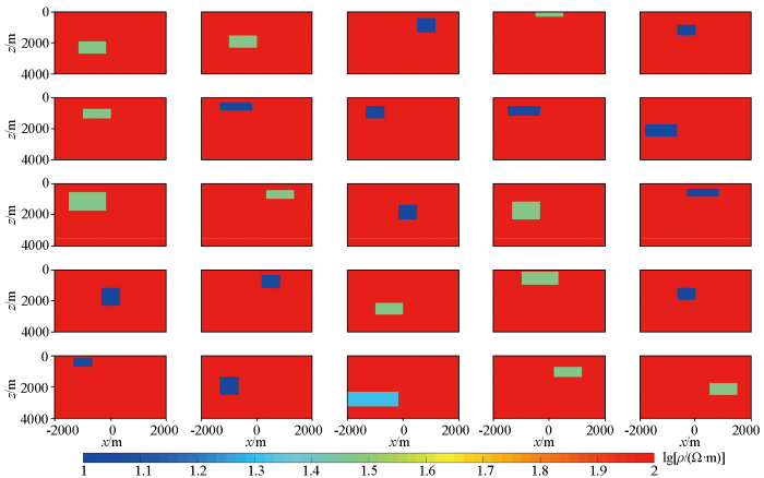
将部分不同电阻率的规则形状的异常体在背景电阻率为100 Ω·m的均匀半空间内移动,形成了4 355个不同模型,如图3所示。

图3

新窗口打开| 下载原图ZIP| 生成PPT

图3 部分训练集

Fig.3 Some training samples

将上述模型分别进行正演计算,使用正演结果中TM模式的数据信息,将上述模型与正演响应构成一个训练集,进行离线训练,本阶段采用matlab及C++混合编程的方法,模型试算工作采用的CPU型号为i5-12500H,开启10线程并行,训练共耗时2 h。

训练过程共迭代8次,初始迭代误差为0.423,迭代8次后误差缩小为0.087。迭代过程如图4所示。从训练集中随机取出80组模型进行验证工作,其中数据误差低于15%的有80组(如图5所示),可见离线训练所求平均下降方向满足反演要求。

图4

新窗口打开| 下载原图ZIP| 生成PPT

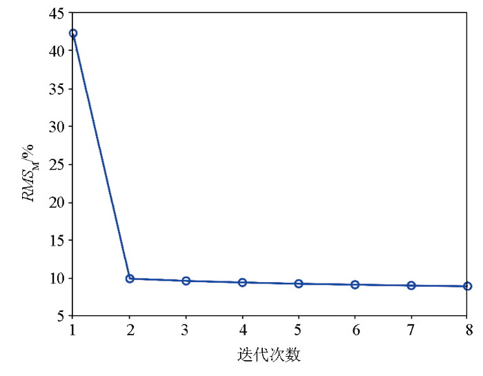
图4 迭代过程的模型拟合差

Fig.4 The normalized model misfit in each iteration during training

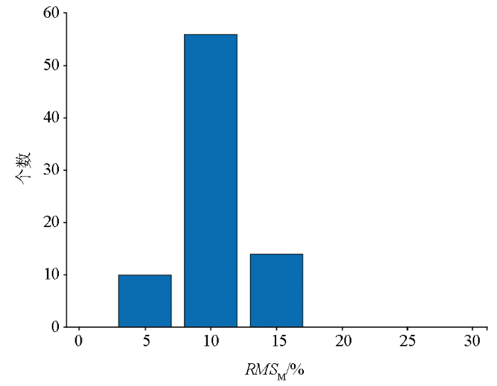
图5

新窗口打开| 下载原图ZIP| 生成PPT

图5 误差分布

Fig.5 The histogram of the normalized model misfit

3.1 理论模型1

模型1(图6)包含4个异常体,背景电阻率为100 Ω·m,异常体1是大小为800 m×800 m、埋深为400 m、电阻率值为1 000 Ω·m的高阻异常体,异常体2是大小为800 m×700 m、埋深为300 m、电阻率值为10 Ω·m的低阻异常体,异常体3是大小为600 m×700 m、埋深为300 m、电阻率值为1 000 Ω·m的高阻异常体,异常体4是大小为1 000 m×1 000 m、埋深为400 m、电阻率值为10 Ω·m的低阻异常体。

图6

新窗口打开| 下载原图ZIP| 生成PPT

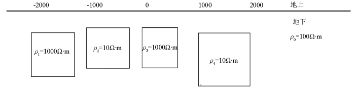
图6 理论模型1示意(从左到右分别为异常体1、2、3、4)

Fig.6 Schematic diagram of model 1 (abnormal bodies 1, 2, 3 and 4 are arranged from left to right)

图7a为模型1正演响应的反演结果,图7b为10%高斯误差合成数据的反演结果,图8为两者的数据拟合曲线。可见,本算法具有一定的抗噪能力。

图7

新窗口打开| 下载原图ZIP| 生成PPT

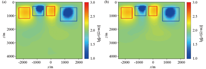
图7 预测结果抗噪能力对比

a—高斯误差为0%的预测结果 ;b—高斯误差为10%的预测结果

Fig.7 Comparison of anti-interference ability

a—inversion results with 0% random noise;b—inversion results with 10% random noise

图8

新窗口打开| 下载原图ZIP| 生成PPT

图8 迭代过程的数据拟合差

Fig.8 The normalized data misfit in iteration

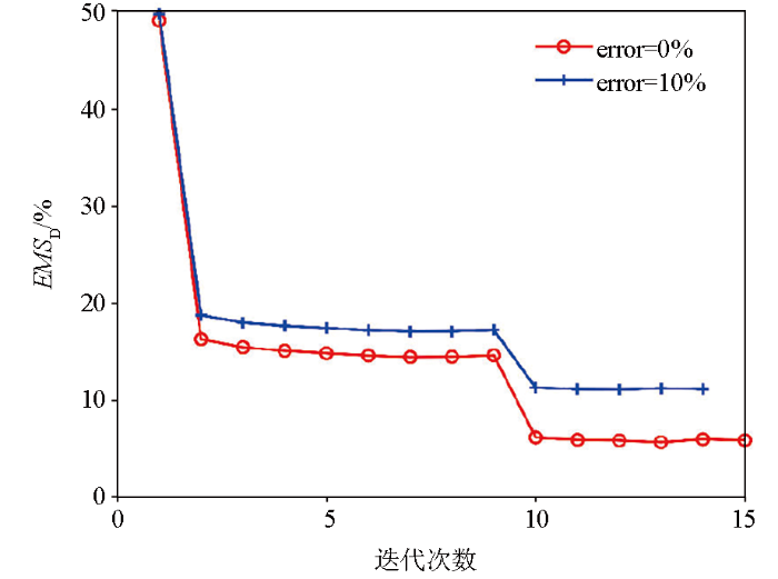
图9a为非线性共轭梯度法的二维反演结果,用时5.695 s。高阻异常体1、3均未能恢复理论模型电阻率,能还原异常体大致位置;低阻异常体2、4未能恢复理论模型电阻率,大致还原异常体位置。

图9

新窗口打开| 下载原图ZIP| 生成PPT

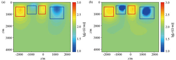
图9 理论模型1反演结果对比

a—非线性共轭梯度反演结果;b—监督下降法反演结果

Fig.9 Comparison of inversion results of model 1

a—inversion results of using NLCG scheme;b——inversion results of using SDM scheme

图9b为监督下降算法反演的结果,用时3.145 s。高阻异常体1、3理论模型电阻率的恢复效果优于图9a,且能够还原异常体位置;低阻异常体2、4的反演结果基本可以恢复理论模型电阻率,也能够还原异常体位置。

3.2 理论模型2

模型2(图10)包含4个异常体,背景电阻率为100 Ω·m,异常体1是大小为1 400 m×1 000 m、埋深为1 200 m、电阻率值为1 000 Ω·m的高阻异常体,异常体2是埋深300 m、电阻率值为10 Ω·m的阶梯状低阻异常体,异常体3是大小为1 200 m×260 m、埋深为40 m、电阻率值为10 Ω·m的低阻异常体,异常体4是大小为600 m×1 300 m、埋深为850 m、电阻率值为1 000 Ω·m的高阻异常体。

图10

新窗口打开| 下载原图ZIP| 生成PPT

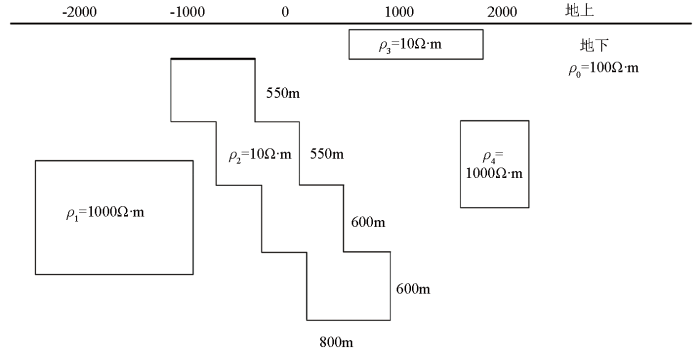
图10 理论模型2示意(从左到右分别为异常体1、2、3、4)

Fig.10 Schematic diagram of model 2 (abnormal bodies 1, 2, 3 and 4 are arranged from left to right)

图11a为非线性共轭梯度法的二维反演的结果,用时5.6 s。高阻异常体1未能恢复理论模型的电阻率,也未能还原异常体位置;非线性共轭梯度反演方法仅恢复了低阻异常体2地下1 000 m以上的信息,但基本无法得出1 000 m以下的有效信息,可能受低阻异常体3的影响较大;低阻异常体3大致恢复理论模型的电阻率,并还原异常体位置;高阻异常体4未恢复理论模型的电阻率,也未还原异常体大致位置。

图11

新窗口打开| 下载原图ZIP| 生成PPT

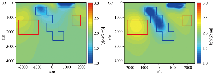
图11 理论模型2反演结果对比

a—非线性共轭梯度反演结果;b—监督下降法反演结果

Fig.11 Comparison of inversion results of model 2

a—inversion results of using NLCG scheme;b—inversion results of using SDM scheme

图11b为监督下降算法反演的结果,初始迭代误差为0.546,迭代10次后迭代误差为0.063 1,用时2.8 s。高阻异常体1理论模型电阻率的恢复效果优于11a,且能还原异常体位置;监督下降算法可以反演出低阻阶梯状异常体2的地下2 000 m以上的异常体信息,并恢复异常体理论模型电阻率,2 000~3 000 m的部分没有很好的体现,可能是低阻异常体3屏蔽的影响;低阻异常体3能恢复理论模型的电阻率,也能还原异常体位置;高阻异常体4理论模型电阻率恢复效果优于11a,可能是低阻异常体3的影响,也未还原异常体位置。

3.3 理论模型3

模型3(图12)为复杂地层模型,背景电阻率为100 Ω·m,存在地层平均层厚500 m,顶部埋深100 m,电阻率值10 Ω·m的中部突起地层异常体。

图12

新窗口打开| 下载原图ZIP| 生成PPT

图12 理论模型3示意

Fig.12 Schematic diagram of model 3

图13a为非线性共轭梯度法的二维反演的结果,用时6.2 s。图13b为监督下降算法反演的结果,初始迭代误差为0.842,迭代10次后迭代误差为0.085,用时3.4 s。监督下降算法的形态更接近真实模型,对异常体的电阻率恢复效果更好。

图13

新窗口打开| 下载原图ZIP| 生成PPT

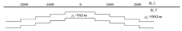
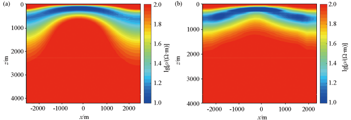
图13 反演结果对比

a—非线性共轭梯度反演结果;b—监督下降法反演结果

Fig.13 Comparison of inversion results

a—inversion results of using NLCG scheme;b—inversion results of using SDM scheme

总体上,监督下降法的反演效果优于非线性共轭梯度法的反演效果。训练集中并没有训练较复杂的模型,但我们仍可以反演理论模型的高阻异常体、复杂异常体以及复杂地层异常模型,说明监督下降法具有处理较复杂模型的能力。

4 实测数据应用

为验证算法的实用性,将本文开发的反演算法应用于西藏高原南部雅鲁藏布江缝合带地区实测数据的反演。测线南起错那县,终止于墨竹工卡县,全长约240 km,测点29个,观测频率范围为0.000 1~250 Hz。测线横跨雅鲁藏布江缝合带,缝合带附近存在大规模的冈底斯花岗岩^[18]。

图14为原始数据拟断面图,本文主要对TM模式的数据进行反演,对比监督下降算法及非线性共轭梯度算法反演结果,以此验证监督下降法的实用性。

图14

新窗口打开| 下载原图ZIP| 生成PPT

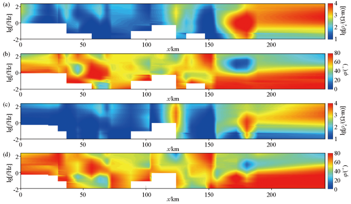
图14 原始数据拟断面(空白区域为剔除的坏点)

a—TM模式视电阻率拟断面;b—TM模式相位拟断面;c—TE模式视电阻率拟断面;d—TE模式相位拟断面

Fig.14 Pseudosection of field data (blank areas indicate removed bad points)

a—apparent resistivity of TM mode;b—impedance phase of TM mode;c—apparent resistivity of TE mode;d—impedance phase of TE mode

图15a为非线性共轭梯度法的反演结果,图15b为监督下降法的反演结果,两者反演结果基本一致。图16为反演结果与实测数据对比,可见大构造拟合程度较高。在时间方面,非线性共轭梯度大致需要30 s,监督下降法的训练时间为2 h左右,预测时间大约25 s。

图15

新窗口打开| 下载原图ZIP| 生成PPT

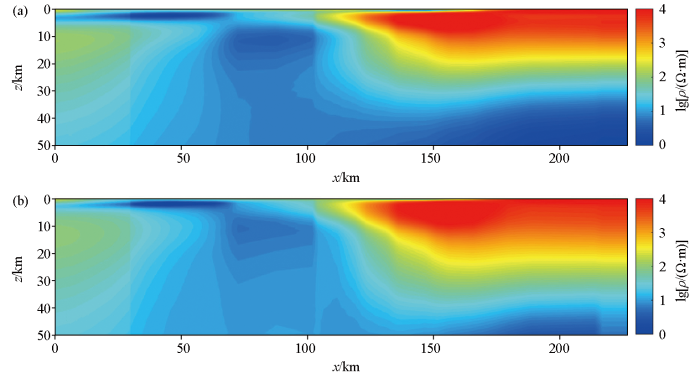
图15 实测数据反演结果对比

a—非线性共轭梯度法反演结果;b—监督下降法的反演结果

Fig.15 Comparison of inversion results of field data

a—inversion results using NLCG scheme;b—inversion results using SDM scheme

图16

新窗口打开| 下载原图ZIP| 生成PPT

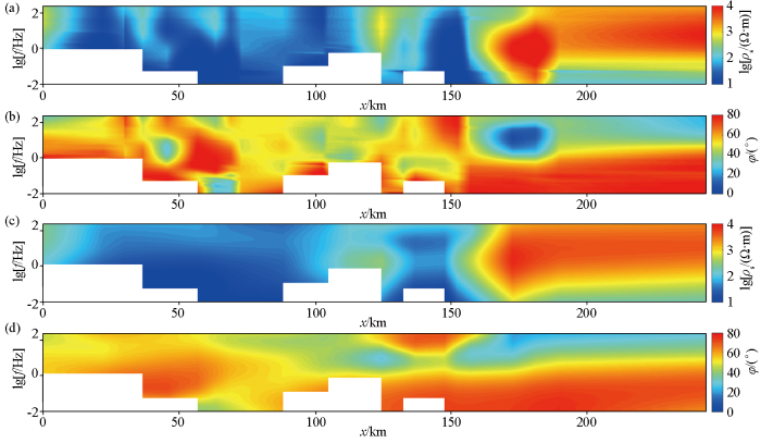
图16 反演结果与实测数据对比

a—原始数据TM模式视电阻率拟断面;b—原始数据TM模式相位拟断面;c—SDM结果TM模式视电阻率拟断面;d—SDM结果TM模式相位拟断面

Fig.16 Comparison of model data and Field data

a—field data apparent resistivity of TM mode;b—field data impedance phase of TM mode;c—SDM inversion results apparent resistivity of TM mode;d—SDM inversion results impedance phase of TM mode

5 结论

本文实现了基于监督下降法的大地电磁二维反演,学习了一组训练集,对三组理论模型和实测数据进行了反演,检验了反演算法的可行性和实用性。反演结果表明基于监督下降法的大地电磁二维反演收敛速度、反演效果优于非线性共轭梯度反演,具有较好的抗噪能力及实用性。

1)训练得到的平均步长对异常体的预测起了指导性作用,避免了雅可比矩阵及海森矩阵的计算,大大降低了陷入局部极小值的风险,减少反演多解性。

2)就预测阶段来说,需要的时间小于常规反演所需的时间,对于批量数据的处理具有一定优势。

3)监督下降法具有较高泛化能力,可以用于更多地球物理勘探方法。

监督下降法总体耗时(训练+预测)较常规反演略长,同时平均步长的储存对硬盘的需求较大,并行降低耗时与减少储存是其未来的研究方向。

参考文献

原文顺序

文献年度倒序

文中引用次数倒序

被引期刊影响因子

[1]

李金铭.

地电场与电法勘探[M]. 武汉: 中国地质大学出版社, 2023.

[本文引用: 1]

J M

Geoelectric field and electric exploration[M]. Wuhan: China University of Geosciences Press, 2023.

[本文引用: 1]

[2]

Avdeeva

Three-dimensional magnetotelluric inversion[D]. Dublin: National University of Ireland, 2008

[本文引用: 1]

[3]

De Groot-Hedlin

, Constable

Occam’s inversion to generate smooth,two-dimensional models from magnetotelluric data

[J]. Geophysics, 1990, 55(12):1613-1624.

DOI:10.1190/1.1442813 URL [本文引用: 1]

Magnetotelluric (MT) data are inverted for smooth 2-D models using an extension of the existing 1-D algorithm, Occam’s inversion. Since an MT data set consists of a finite number of imprecise data, an infinity of solutions to the inverse problem exists. Fitting field or synthetic electromagnetic data as closely as possible results in theoretical models with a maximum amount of roughness, or structure. However, by relaxing the misfit criterion only a small amount, models which are maximally smooth may be generated. Smooth models are less likely to result in overinterpretation of the data and reflect the true resolving power of the MT method. The models are composed of a large number of rectangular prisms, each having a constant conductivity. [Formula: see text] information, in the form of boundary locations only or both boundary locations and conductivity, may be included, providing a powerful tool for improving the resolving power of the data. Joint inversion of TE and TM synthetic data generated from known models allows comparison of smooth models with the true structure. In most cases, smoothed versions of the true structure may be recovered in 12–16 iterations. However, resistive features with a size comparable to depth of burial are poorly resolved. Real MT data present problems of non‐Gaussian data errors, the breakdown of the two‐dimensionality assumption and the large number of data in broadband soundings; nevertheless, real data can be inverted using the algorithm.

[4]

Egbert

G D

, Kelbert

Computational recipes for electromagnetic inverse problems

[J]. Geophysical Journal International, 2012, 189(1):251-267.

DOI:10.1111/gji.2012.189.issue-1 URL [本文引用: 1]

[5]

You

, Zhou

, Ding

L Y

Deep learning technology for construction machinery and robotics

[J]. Automation in Construction, 2023, 150:104852.

DOI:10.1016/j.autcon.2023.104852 URL [本文引用: 1]

[6]

Ding

J Q

, Xu

, Nguyen

M T

, et al.

Machine learning for molecular thermodynamics

[J]. Chinese Journal of Chemical Engineering, 2021, 31(3):227-239.

DOI:10.1016/j.cjche.2020.10.044 URL [本文引用: 1]

[7]

Xiong

X H

, De la Torre

Supervised descent method and its applications to face alignment

[C]// 2013 IEEE Conference on Computer Vision and Pattern Recognition.Portland,OR,USA.IEEE, 2013:532-539.

[本文引用: 1]

[8]

Xiong

, De-la-Torre

, et al.

Supervised descent method(Conference Paper)

[J]. Proceedings of the IEEE Computer Society Conference on Computer Vision and Pattern Recognition, 2015(7):2664-2673

[本文引用: 1]

[9]

Zhang

, Guo

, Zhang

H L

, et al.

Image human thorax using ultrasound traveltime tomography with supervised descent method

[J]. Applied Sciences, 2022, 12(13):6763.

DOI:10.3390/app12136763 URL [本文引用: 1]

The change of acoustic velocity in the human thorax reflects the functional status of the respiratory system. Imaging the thorax’s acoustic velocity distribution can be used to monitor the respiratory system. In this paper, the feasibility of imaging the human thorax using ultrasound traveltime tomography with a supervised descent method (SDM) is studied. The forward modeling is computed using the shortest path ray tracing (SPR) method. The training model is composed of homogeneous acoustic velocity background and a high-velocity rectangular block moving in the domain of interest (DoI). The average descent direction is learned from the training set. Numerical experiments are conducted to verify the method’s feasibility. Normal thorax model experiment proves that SDM traveltime tomography can efficiently reconstruct thorax acoustic velocity distribution. Numerical experiments based on synthetic thorax model of pleural effusion and pneumothorax show that SDM traveltime tomography has good generalization ability and can detect the change of acoustic velocity in human thorax. This method might be helpful for the diagnosis and evaluation of respiratory diseases.

[10]

Lin

, Liu

Guided wave tomography based on supervised descent method for quantitative corrosion imaging

[J]. IEEE Transactions on Ultrasonics,Ferroelectrics,and Frequency Control, 2021, 68(12):3624-3636.

DOI:10.1109/TUFFC.2021.3097080 URL [本文引用: 1]

[11]

Guo

, Jia

Z K

, Song

X Q

, et al.

Pixel- and model-based microwave inversion with supervised descent method for dielectric targets

[J]. IEEE Transactions on Antennas and Propagation, 2020, 68(12):8114-8126.

DOI:10.1109/TAP.8 URL [本文引用: 1]

[12]

Guo

, Li

M K

, Yang

, et al.

Application of supervised descent method for 2D magnetotelluric data inversion

[J]. Geophysics, 2020, 85(4):WA53-WA65.

DOI:10.1190/geo2019-0409.1 URL [本文引用: 1]

The supervised descent method (SDM) is applied to 2D magnetotellurics (MT) data inversion. SDM contains offline training and online prediction. The training set is composed of the models generated according to prior knowledge and the data simulated by MT forward modeling. In the training process, a set of descent directions from an initial model to the training models is learned. In the prediction, model reconstruction is achieved by optimizing an online regularized objective function with a restart scheme, where the learned descent directions and the computed data residual are involved. SDM inversion has the advantages of (1) being more efficient than traditional gradient-descent methods because the computation of local derivatives of the objective function is avoided, (2) incorporating prior uncertain knowledge easier than deterministic inversion approach by generating training models flexibly, and (3) having high generalization ability because the physical modeling can guide the online model reconstruction. Furthermore, a way of designing general training set is introduced, which can be used for training when the prior knowledge is weak. The efficiency and accuracy of this method are validated by two numerical examples. The results indicate that the reconstructed models are consistent with prior information, and the simulated responses agree well with the data. This method also shows good potential to improve the accuracy and efficiency in field MT data inversion.

[13]

Guo

, Li

M K

, Fang

G Y

, et al.

Application of supervised descent method to transient electromagnetic data inversion

[J]. Geophysics, 2019, 84(4):E225-E237.

DOI:10.1190/geo2018-0129.1 URL [本文引用: 1]

Inversion plays an important role in transient electromagnetic (TEM) data interpretation. This problem is highly nonlinear and severely ill posed. Gradient-descent methods have been widely used to invert TEM data, and regularization schemes containing prior information are applied to reduce the nonuniqueness and stabilize the inversion. During the inversion, the partial derivatives are repeatedly computed, which is time and memory consuming. Furthermore, regularization schemes can only provide limited prior information. Much prior information from knowledge and experience cannot be directly used in inversion. In this work, we applied the supervised descent method (SDM) to TEM data inversion. This method contains an offline training stage and an online prediction stage. In the training stage, a training data set is generated according to prior information. Then, the average descent direction between a fixed initial model and the training models can be learned by iterative schemes. In the online stage of prediction, the learned descent directions are applied directly into the inversion to update the models. In this manner, one can select models satisfying the data and model misfit. In this study, SDM is applied to model- and pixel-based inversion schemes. Synthetic examples indicate that SDM inversion can not only enhance the accuracy of inversion due to the incorporation of prior information but also largely accelerate the inversion procedure because it avoids the online computation of derivatives.

[14]

余年.

大地电磁二、三维倾子正演模拟与联合反演研究[D]. 成都: 成都理工大学, 2012.

[本文引用: 1]

2D/3D tipper forward modeling and joint inversion of magnetotelluric[D]. Chengdu: Chengdu University of Technology, 2012.

[本文引用: 1]

[15]

林昌洪.

大地电磁张量阻抗三维共轭梯度反演研究[D]. 北京: 中国地质大学(北京), 2009.

[本文引用: 1]

Lin

C H

Three-dimensional conjugate gradients inversion of magnetotelluric impedance tensor[D]. Beijing: China University of Geosciences(Beijing), 2009.

[本文引用: 1]

[16]

Newman

G A

, Alumbaugh

D L

Three-dimensional magnetotelluric inversion using non-linear conjugate gradients

[J]. Geophysical Journal International, 2000, 140(2):410-424.

DOI:10.1046/j.1365-246x.2000.00007.x URL [本文引用: 1]

[17]

翁爱华, 刘云鹤, 贾定宇, 等.

地面可控源频率测深三维非线性共轭梯度反演

[J]. 地球物理学报, 2012, 55(10):3506-3515.

[本文引用: 1]

Weng

A H

, Liu

Y H

, Jia

D Y

, et al.

Three-dimensional controlled source electromagnetic inversion using non-linear conjugate gradients

[J]. Chinese Journal of Geophysics, 2012, 55(10):3506-3515.

[本文引用: 1]

[18]

谭捍东, 魏文博, Martyn

Unsworth

, 等.

西藏高原南部雅鲁藏布江缝合带地区地壳电性结构研究

[J]. 地球物理学报, 2004, 47(4):685-690.

[本文引用: 1]

Tan

H D

, Wei

W B

, Unsworth

, et al.

Crustal electrical conductivity structure beneath the Yarlung Zangbo Jiang suture in the southern Xizang Plateau

[J]. Chinese Journal of Geophysics, 2004, 47(4):685-690.

[本文引用: 1]

2023

... 大地电磁测深法(MT)是一种通过观测天然交变电磁场来对地电构造进行研究的物探方法,大地电磁法的频域很宽,其探测深度距地表有几百米到数百公里不等,具有分辨率高,穿透能力强,勘探深度大以及效率高等实际优点,被广泛应用于金属矿产普查、勘探地热和油气田等领域^[1]. ...

2023

2008

... 大地电磁二维反演常采用高斯牛顿法^[2]、OCCAM法^[3]、非线性共轭梯度法^[4]等,这些方法在最小化目标函数时各有优劣,但都无法在迭代过程中避免雅可比矩阵或海森矩阵的计算,且存在陷入局部极小值的风险,导致反演效果变差. ...

Occam’s inversion to generate smooth,two-dimensional models from magnetotelluric data

1990

Computational recipes for electromagnetic inverse problems

2012

Deep learning technology for construction machinery and robotics

2023

... 近些年随着计算机行业的发展,机器学习成功在多种领域取得不错的效果^[5].机器学习能够挖掘变量与标签之间的关联,并学习其关联进行预测,大大减少反演时间,提升计算效率^[6]. ...

Machine learning for molecular thermodynamics

2021

Supervised descent method and its applications to face alignment

2013

... 监督下降法(SDM)在人脸识别技术中被广泛使用^[7-8],后被带入到多领域进行研究^[9⇓-11].采取监督下降法解决地球物理勘探领域的问题也取得了不错的成效^[12],模型与正演响应合并构成的训练集在进行一维瞬变电磁(TEM)反演中发挥了重要的作用^[13].监督下降法分为离线训练和在线预测两个阶段,在离线训练阶段,通过学习大量模型及其响应得出平均下降步长.在预测阶段,采用学习的步长进行迭代预测.平均步长具有较好的指导作用,避免了迭代陷入局部极小的风险,提升了反演的效果.此外,监督下降法并不需要计算雅可比矩阵和海森矩阵,避免了内存浪费的同时,提升了反演的效率. ...

Supervised descent method(Conference Paper)

2015

Image human thorax using ultrasound traveltime tomography with supervised descent method

2022

Guided wave tomography based on supervised descent method for quantitative corrosion imaging

2021

Pixel- and model-based microwave inversion with supervised descent method for dielectric targets

2020

Application of supervised descent method for 2D magnetotelluric data inversion

2020

Application of supervised descent method to transient electromagnetic data inversion

2019

2012

... 式中:k为波数,k=

\sqrt[]{- i ω μ_{0} σ}

,大地电磁二维有限单元正演的变分问题为^[14]: ...

2012

... 式中:k为波数,k=

\sqrt[]{- i ω μ_{0} σ}

,大地电磁二维有限单元正演的变分问题为^[14]: ...

2009

... 定义大地电磁二维反演目标函数如下^[15]: ...

2009

... 定义大地电磁二维反演目标函数如下^[15]: ...

Three-dimensional magnetotelluric inversion using non-linear conjugate gradients

2000

... 非线性共轭梯度反演的具体步骤如下^[16-17]: ...

地面可控源频率测深三维非线性共轭梯度反演

2012

... 非线性共轭梯度反演的具体步骤如下^[16-17]: ...

地面可控源频率测深三维非线性共轭梯度反演

2012

... 非线性共轭梯度反演的具体步骤如下^[16-17]: ...

西藏高原南部雅鲁藏布江缝合带地区地壳电性结构研究

2004

... 为验证算法的实用性,将本文开发的反演算法应用于西藏高原南部雅鲁藏布江缝合带地区实测数据的反演.测线南起错那县,终止于墨竹工卡县,全长约240 km,测点29个,观测频率范围为0.000 1~250 Hz.测线横跨雅鲁藏布江缝合带,缝合带附近存在大规模的冈底斯花岗岩^[18]. ...

西藏高原南部雅鲁藏布江缝合带地区地壳电性结构研究

2004

〈

〉