

0 引言
频散曲线反演隶属地球物理反演问题范畴,具有高度非线性、多参数、多极值的特点[3-4]。同时由于地震数据存在噪声、反演多解性等因素的影响,想要精确且高效地反演频散曲线变得非常困难。频散曲线的反演算法可分为局部优化算法和全局优化算法。局部优化算法有最小二乘法[5⇓⇓⇓-9]、L-M算法[10]、Occam算法[11-12]等。早期,局部优化算法因计算速度快而被广泛应用。但此类方法过度依赖于初始模型的建立,初始模型选取和真实情况相近才能获得较好的反演效果。另外,算法易陷入局部极值,并且涉及到的偏导数计算以及反演结果的好坏都受到雅可比矩阵精度的影响[13-14]。这些使局部优化算法在瑞利波反演领域的发展受到限制。另一种全局优化算法因可以很好地避免局部优化算法在反演时遇到的问题,受到学者们的广泛关注。全局优化算法中常用的有遗传算法[15⇓-17]、模拟退火算法[18⇓⇓⇓-22]、粒子群算法等[23-24]。这些算法和局部优化算法相比虽具有不依赖于初始模型、不易陷入局部最优解等优势,但存在运算时间长、容易早熟收敛等缺点。
鉴于此,本文将一种新的正余弦算法(sine cosine algorithm,SCA)用于瑞利波频散曲线的反演研究。为了评价SCA对瑞利波频散曲线反演的可行性、有效性、稳定性和实用性,本文首先利用SCA对4个从简单到复杂的地质模型产生的含噪声与不含噪声的理论频散曲线进行反演,并分析与评价SCA的可行性,有效性和稳定性。接着,通过进一步对比SCA与PSO的反演性能以说明SCA相对于经典的粒子群算法是否具有更稳定、收敛速度更快,反演精度更高的优越性。最后将SCA用于反演来自冰岛Arnarbælidi和美国怀俄明地区的实测数据以检验SCA对瑞利波频散曲线反演的实用性。
1 SCA基本原理
SCA是澳洲学者Seyedali Mirjalili在基于正余弦函数组合,应用多个随机参数和自适应变量调整寻优过程的基础上于2016年提出的一种新型群智能优化算法[25]。SCA与其他群智能优化算法相同,可以根据先验信息给出每个解的初始值。如果先验信息不可用,则可以随机生成初始集合。然后这些解的位置更新方程如下:
式中:
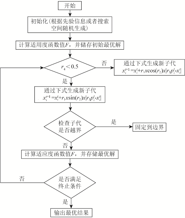
式中:t为当前迭代次数;T为最大迭代次数;a为一常量。图1给出了SCA的算法流程。
图1
2 理论模型测试
在实际工程应用中,基阶频散曲线能量更强,更易观测,采集数据中大多只含有基阶信息,所以在反演时一般选取基阶频散曲线进行反演[26]。本文考虑到出现高阶频散的情况,对基阶、高阶频散曲线联合反演的情况也进行了测试。在测试中将所有地层信息都设为未知,即同时反演厚度、密度、横波速度以及纵波速度,最后选取对频散曲线有显著影响的层厚和横波速度来进行分析与评价。由于真实的地层情况比较复杂,将模型参数的搜索范围设置为真实模型的50%。对于算法参数设置,SCA中影响算法性能的参数主要为种群数和迭代次数。本文设置SCA的种群数为30,迭代次数为100。为避免算法的随机性,每次理论模型测试都进行独立反演30次,且每次反演初始模型都不相同,最后将30次反演所得数据的均值作为反演结果进而输出,标准差作为衡量算法稳定性的指标进而评价。
瑞利波频散曲线反演的本质是求解适应度函数最小值的优化问题。本文采用的适应度函数是根据反演所得模型能否精确解释观测资料所定[27]:
式中:
表1 模型参数及反演搜索范围
Table 1
| 模型 | 层序号 | 模型参数 | 搜索范围 | ||||||||||||||||||
|---|---|---|---|---|---|---|---|---|---|---|---|---|---|---|---|---|---|---|---|---|---|
| vs/(m·s-1) | vp/(m·s-1) | ρ/(g·cm-3) | h/m | vs/(m·s-1) | h/m | ||||||||||||||||
| 模型A | 1 | 200 | 780 | 1.9 | 5 | 100~300 | 2.5~7.5 | ||||||||||||||
| 均匀半空间 | 350 | 850 | 1.9 | ∞ | 175~525 | ∞ | |||||||||||||||
| 模型B | 1 | 200 | 663 | 1.9 | 2 | 100~300 | 1~3 | ||||||||||||||
| 2 | 300 | 995 | 1.9 | 4 | 150~450 | 2~6 | |||||||||||||||
| 3 | 400 | 1327 | 1.9 | 6 | 200~600 | 3~9 | |||||||||||||||
| 均匀半空间 | 500 | 1658 | 1.9 | ∞ | 250~750 | ∞ | |||||||||||||||
| 模型C | 1 | 200 | 663 | 1.9 | 2 | 100~300 | 1~3 | ||||||||||||||
| 2 | 160 | 673 | 1.9 | 4 | 80~240 | 2~6 | |||||||||||||||
| 3 | 300 | 1102 | 1.9 | 6 | 150~450 | 3~9 | |||||||||||||||
| 均匀半空间 | 400 | 1470 | 1.9 | ∞ | 200~600 | ∞ | |||||||||||||||
| 模型D | 1 | 150 | 498 | 1.9 | 2 | 75~225 | 1~3 | ||||||||||||||
| 2 | 250 | 829 | 1.9 | 4 | 125~375 | 2~6 | |||||||||||||||
| 3 | 200 | 841 | 1.9 | 6 | 100~300 | 3~9 | |||||||||||||||
| 均匀半空间 | 400 | 1470 | 1.9 | ∞ | 200~600 | ∞ | |||||||||||||||
2.1 无噪声数据反演
图2
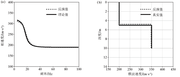
图2
模型A不含噪声理论数据反演结果
a—反演所得频散曲线;b—反演的横波速度剖面
Fig.2
Inversion results of noise-free data of model A
a—inverted response compared with the original one;b—inverted shear-wave velocity profile
表2 模型A、B、C、D含噪声与不含噪声反演结果
Table 2
| 模型 | 参数 | 真实值 | 不含噪声 | 含噪声 | |||||||||||
|---|---|---|---|---|---|---|---|---|---|---|---|---|---|---|---|
| 反演均值 | 相对误差/% | 标准差 | 反演均值 | 相对误差/% | 标准差 | ||||||||||
| 模型A | vs1/(m·s-1) | 200 | 199.54 | 0.23% | 1.28 | 199.69 | 0.15% | 2.71 | |||||||
| vs2/(m·s-1) | 350 | 347.90 | 0.60% | 5.98 | 350.79 | 0.23% | 9.07 | ||||||||
| H1/m | 5 | 4.76 | 4.76% | 0.18 | 4.75 | 5.00% | 0.22 | ||||||||
| 模型B | vs1/(m·s-1) | 200 | 200.94 | 0.47% | 2.52 | 200.95 | 0.47% | 3.82 | |||||||
| vs2/(m·s-1) | 300 | 300.75 | 0.25% | 7.42 | 304.07 | 1.36% | 15.60 | ||||||||
| vs3/(m·s-1) | 400 | 399.19 | 0.20% | 9.34 | 391.88 | 2.03% | 25.47 | ||||||||
| vs4/(m·s-1) | 500 | 500.19 | 0.04% | 6.03 | 499.62 | 0.08% | 6.80 | ||||||||
| H1/m | 2 | 2.05 | 2.52% | 0.11 | 2.02 | 0.83% | 0.16 | ||||||||
| H2/m | 4 | 3.99 | 0.24% | 0.28 | 3.96 | 1.12% | 0.18 | ||||||||
| H3/m | 6 | 5.59 | 6.76% | 0.53 | 5.61 | 6.54% | 0.97 | ||||||||
| 模型C | vs1/(m·s-1) | 200 | 197.78 | 1.11% | 9.25 | 199.90 | 0.05% | 14.71 | |||||||
| vs2/(m·s-1) | 160 | 161.15 | 0.72% | 4.52 | 160.55 | 0.34% | 5.35 | ||||||||
| vs3/(m·s-1) | 300 | 286.04 | 4.65% | 32.13 | 285.78 | 4.74% | 22.89 | ||||||||
| vs4/(m·s-1) | 400 | 397.61 | 0.60% | 13.58 | 397.19 | 0.70% | 18.96 | ||||||||
| H1/m | 2 | 1.97 | 1.57% | 0.17 | 1.91 | 4.51% | 0.23 | ||||||||
| H2/m | 4 | 3.86 | 3.58% | 0.43 | 3.85 | 3.71% | 0.30 | ||||||||
| H3/m | 6 | 5.62 | 6.28% | 1.09 | 5.51 | 8.16% | 0.43 | ||||||||
| 模型D | vs1/(m·s-1) | 150 | 150.58 | 0.39% | 1.03 | 149.80 | 0.13% | 2.92 | |||||||
| vs2/(m·s-1) | 250 | 252.30 | 0.92% | 4.25 | 251.41 | 0.56% | 7.38 | ||||||||
| vs3/(m·s-1) | 200 | 199.81 | 0.09% | 3.94 | 202.01 | 1.01% | 4.41 | ||||||||
| vs4/(m·s-1) | 400 | 400.90 | 0.23% | 4.80 | 400.46 | 0.12% | 6.36 | ||||||||
| H1/m | 2 | 2.03 | 1.41% | 0.07 | 2.03 | 1.36% | 0.08 | ||||||||
| H2/m | 4 | 3.93 | 1.78% | 0.14 | 3.98 | 0.44% | 0.24 | ||||||||
| H3/m | 6 | 6.09 | 1.45% | 0.23 | 5.99 | 0.14% | 0.26 | ||||||||
图3
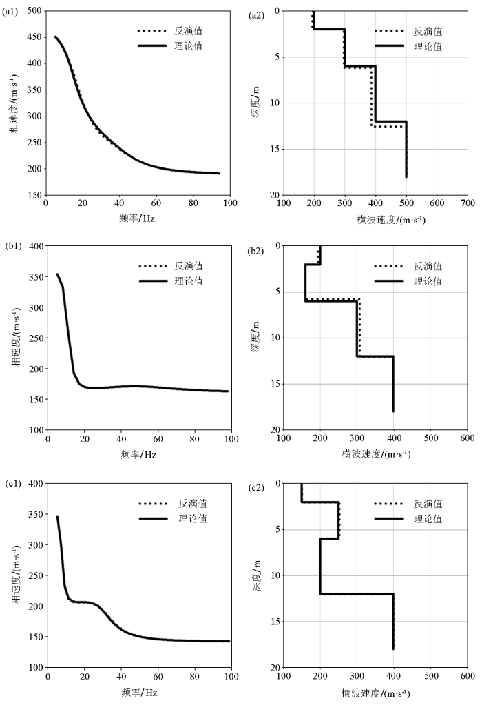
图3
模型B、C和D不含噪声理论数据反演结果
a1,b1,c1—分别为模型B、C和D反演所得频散曲线;a2,b2,c2—分别为模型B、C和D反演的横波速度剖面
Fig.3
Inversion results of noise-free data of model B,C,and D
a1,b1,c1—inverted dispersion curves obtained from model B,C and D respectively;a2,b2,c2—inverted shear-wave velocity profiles obtained from model B,C and D respectively
2.2 含噪声数据反演
在采集地震数据时,噪声是难以避免的。这些噪声会使提取到的频散曲线在小范围内随机扰动,进而影响反演结果。因此,算法用于实际数据处理前需检测其抗噪能力。为测试SCA的抗噪性能,在以上4个理论模型经正演模拟得到的频散曲线中加入15%的随机噪声后进行反演。
图4
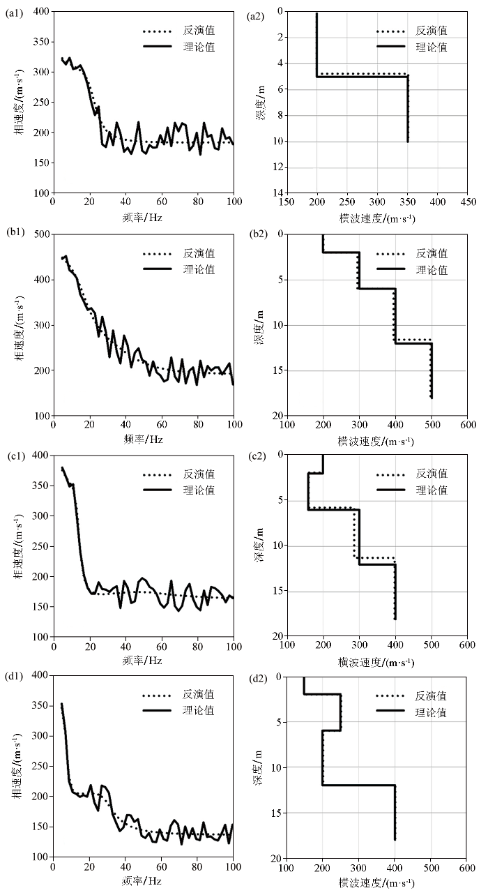
图4
模型A、B、C、D的含噪声理论数据反演结果
a1,b1,c1,d1—分别为模型A、B、C和D反演所得频散曲线;a2,b2,c2,d2—分别为模型A、B、C和D反演的横波速度剖面
Fig.4
Inversion results of noise-contaminated data of model A,B,C,and D
a1,b1,c1,d1—inverted dispersion curves obtained from model A,B,C and D respectively;a2,b2,c2,d2—inverted shear-wave velocity profiles obtained from model A,B,C and D respectively
2.3 多模式频散曲线反演
在一些特殊地层(如软弱夹层),可能会出现高阶波高频部分能量强于基阶波的情况[28],这时若将高阶频散曲线和基阶频散曲线联合起来反演,便可以增加反演的有效信息,进而提升反演所得地层信息的准确度,故检验算法对于多模式频散曲线的反演能力是必要的。此次测试以模型C为例,向模型C的基阶频散曲线数据中加入高阶数据后进行反演试算,反演结果见图5和表3。从图5a1可知,反演得到的频散曲线(点线),无论基阶还是高阶,都与真实模型频散曲线(实线)拟合得很好并且由图5a2可看出,反演所得模型参数(点线)与真实模型参数(实线)相差也较小,说明SCA用于多模式频散曲线反演是可行的。另外,多模式频散曲线反演结果相比单纯基阶频散曲线反演结果的精度总体有所提升,尤其是第三层层厚的相对误差从6.28%降到了1.38%。由此可知,多模式频散曲线反演比只用基阶频散曲线进行反演所得模型参数准确度更高,反演效果更优异。
图5
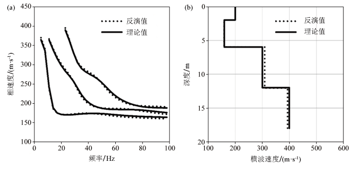
图5
模型C多模式数据反演结果
a—反演所得频散曲线;b—反演的横波速度剖面
Fig.5
Inversion results of model C with multi-modal data
a—inverted responses compared with the original ones;b—inverted shear-wave velocity profile
表3 模型C基阶数据和多模式数据反演结果
Table 3
| 参数 | 真实值 | 基阶数据 | 多模数据 | ||||
|---|---|---|---|---|---|---|---|
| 反演均值 | 相对误差/% | 标准差 | 反演均值 | 相对误差/% | 标准差 | ||
| vs1/(m·s-1) | 200 | 197.78 | 1.11% | 9.25 | 200.18 | 0.09% | 9.75 |
| vs2/(m·s-1) | 160 | 161.15 | 0.72% | 4.52 | 158.98 | 0.64% | 4.60 |
| vs3/(m·s-1) | 300 | 286.04 | 4.65% | 32.13 | 308.08 | 2.93% | 21.04 |
| vs4/(m·s-1) | 400 | 397.61 | 0.60% | 13.58 | 393.26 | 1.68% | 15.64 |
| H1/m | 2 | 1.97 | 1.57% | 0.17 | 1.99 | 0.70% | 0.23 |
| H2/m | 4 | 3.86 | 3.58% | 0.43 | 3.99 | 0.28% | 0.30 |
| H3/m | 6 | 5.62 | 6.28% | 1.09 | 6.08 | 1.38% | 0.43 |
3 同粒子群算法的对比
为证实SCA用于频散曲线反演确实能得到较为准确的地层参数,将其和经典的粒子群算法(particle swarm optimization,PSO)一起进行反演测试,对比、分析和评价两者的反演性能。测试在不含噪声的模型D上进行,各单独反演30次。反演时两种算法的种群数目,搜索空间和迭代次数都相同。反演结果如图6所示,具体的反演参数如表4所示。结合图6a2和表4可知,SCA在迭代初期就大致确定了最优解位置,迭代到30次的时候就基本收敛且收敛精度较高为1.35 m/s;PSO的寻优能力较差,在迭代到40次左右才收敛并且在100次左右时还有进一步收敛的趋势,最后收敛的精度也较低为11.57 m/s。除此之外,通过表4中SCA与PSO对于模型各参数反演的标准差可以看到,SCA算法的稳定性远远强于传统的粒子群算法,这得益于SCA独特的更新解的方式。综上可知SCA相较于PSO在瑞雷波频散曲线反演中的表现具有更高的精度,更快的收敛速度以及更强的稳定性。
图6
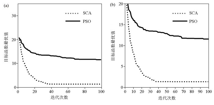
图6
SCA与PSO在无噪声模型D中反演收敛过程对比
a—放大前的收敛曲线对比;b—放大后的收敛曲线对比
Fig.6
Comparison of the convergence rate between SCA and PSO on noise-free data from model D
a—comparison of convergence curves before zooming up;b—comparison of convergence curves after zooming up
表4 SCA和PSO反演效果对比
Table 4
| 参数 | 真实值 | SCA | PSO | ||||
|---|---|---|---|---|---|---|---|
| 反演均值 | 相对误差/% | 标准差 | 反演均值 | 相对误差/% | 标准差 | ||
| vs1/(m·s-1) | 150 | 150.58 | 0.39% | 1.03 | 148.06 | 1.29% | 9.91 |
| vs2/(m·s-1) | 250 | 252.30 | 0.92% | 4.25 | 242.06 | 3.18% | 23.34 |
| vs3/(m·s-1) | 200 | 199.81 | 0.09% | 3.94 | 176.28 | 11.86% | 37.69 |
| vs4/(m·s-1) | 400 | 400.90 | 0.23% | 4.80 | 374.89 | 6.28% | 27.63 |
| H1/m | 2 | 2.03 | 1.41% | 0.07 | 1.93 | 3.5% | 0.38 |
| H2/m | 4 | 3.93 | 1.78% | 0.14 | 3.72 | 6.86% | 0.97 |
| H3/m | 6 | 6.09 | 1.45% | 0.23 | 4.07 | 32.14% | 2.03 |
4 实际资料测试
图7
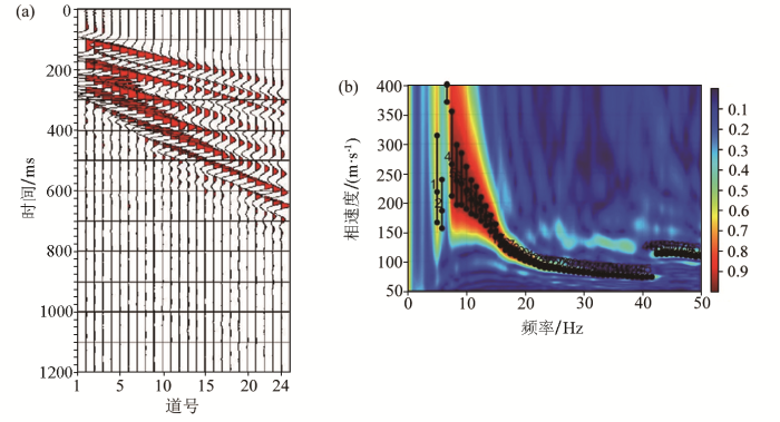
表5 Arnarbælidi地区前人[29]反演模型参数以及搜索范围[30]
Table 5
| 文献估计层厚 | 文献S波速度 | S波速度搜索范围 | 厚度搜索范围 |
|---|---|---|---|
| /m | /(m·s-1) | /(m·s-1) | /m |
| 0.8 | 78 | 60~90 | 0.1~1.5 |
| 0.5 | 80 | 70~100 | 0.1~1.5 |
| 0.7 | 92 | 80~110 | 0.1~1.5 |
| 1.2 | 111 | 100~150 | 0.5~2.0 |
| 1.9 | 141 | 120~200 | 0.5~2.0 |
| 3.0 | 184 | 150~250 | 2.0~4.0 |
| 4.7 | 230 | 200~300 | 3.0~5.5 |
| 7.5 | 277 | 250~350 | 6.0~9.0 |
| 5.2 | 350 | 300~400 | 4.0~6.0 |
| ∞ | 350 | 320~450 | ∞ |
图8

图8
Arnarbælidi地区瑞雷波相速度反演结果
a—反演所得频散曲线;b—最小目标函数值随迭代次数变化情况;c—反演的横波速度剖面
Fig.8
Inversion results in Arnarbælidi region
a—inverted response compared with the original one;b—the minimum value of the objective function changes with the number of iterations;c—inverted shear-wave velocity profile
图9
| 层数 | vs/(m·s-1) | h/m | 泊松比 | ρ/(g·cm-3) |
|---|---|---|---|---|
| 1 | 100~300 | 1~5 | 0.38 | 2.0 |
| 2 | 100~400 | 1~5 | 0.38 | 2.0 |
| 3 | 100~600 | 1~5 | 0.35 | 2.0 |
| 4 | 200~600 | 1~5 | 0.35 | 2.0 |
| 5 | 200~800 | 均匀半空间 | 0.30 | 2.0 |
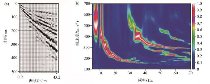
图10
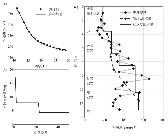
图10
怀俄明地区瑞利波相速度反演结果
a—反演所得频散曲线;b—最小目标函数值随迭代次数变化情况;c—测井数据与反演横波速度剖面对比
Fig.10
Inversion results in Wyoming region
a—inverted response compared with the original one;b—the minimum value of the objective function changes with the number of iterations;c—comparison of the logging data and the inverted shear-wave velocity profile
5 结论
本文将一种新的群智能优化算法——SCA用于瑞利波频散曲线反演的研究当中。在进行具体的反演工作时,通过设置较大的模型参数搜索范围以模拟无先验信息或者仅有少量已知信息的情况,并同时反演厚度、密度、横波速度以及纵波速度以更好适应真实情况(但只选取对频散曲线有显著影响的层厚和横波速度来进行分析与评价)。利用多个理论模型(从简单模型到复杂模型,从无噪声数据到含噪声数据)对SCA性能从理论的角度进行了详尽的测试,最后再采用来自冰岛Arnarbælidi和美国怀俄明地区的实测数据检验了SCA的实用性。测试结果表明:
1)基于正余弦函数组合,应用多个随机参数和自适应变量调整寻优过程的SCA对于频散曲线反演搜索空间具有十分优异的探索和开发能力,在获得高精度地层模型参数的同时还保证了收敛速度以及较强的稳定性,具有良好的发展潜力。
2)SCA相较于传统的粒子群算法在瑞利波频散曲线反演中的表现具有更高的精度、更快的收敛速度以及更强的稳定性。
参考文献
面波勘探技术的研究现状及进展
[J].
Research status and progress of surface wave exploration technology
[J].
基于互相关相移的主动源地震面波频散成像方法
[J].
Activeseismic surface wave dispersion imaging method based on cross-correlation and phase-shifting
[J].
Rayleigh wave dispersion curve inversion via genetic algorithms and marginal posterior probability density estimation
[J].DOI:10.1016/j.jappgeo.2006.04.002 URL [本文引用: 1]
Nonlinear Rayleigh wave inversion based on the shuffled frog-leaping algorithm
[J].DOI:10.1007/s11770-017-0641-x [本文引用: 1]
Numerical inversion of seismic surface wave dispersion data and crust-mantle structure in the New York—Pennsylvania area
[J].DOI:10.1029/JZ067i013p05227 URL [本文引用: 1]
In situ measurements of shear-wave velocity in sediments with higher-mode Rayleigh waves
[J].DOI:10.1111/gpr.1987.35.issue-2 URL [本文引用: 1]
近地表低速带反演
[J].
Near surface low velocity zone inversion
[J].
Automated inversion procedure for spectral analysis of surface waves
[J].DOI:10.1061/(ASCE)1090-0241(1998)124:8(757) URL [本文引用: 1]
用等厚薄层权重自适应迭代阻尼最小二乘法反演瑞雷波频散曲线
[J].
The inversion of dispersion curves using self-adaptively iterative damping least square method by combining equal thinner layers with weighting matrix
[J].
Estimation of near-surface shear-wave velocity by inversion of Rayleigh waves
[J].
DOI:10.1190/1.1444578
URL
[本文引用: 1]

The shear‐wave (S-wave) velocity of near‐surface materials (soil, rocks, pavement) and its effect on seismic‐wave propagation are of fundamental interest in many groundwater, engineering, and environmental studies. Rayleigh‐wave phase velocity of a layered‐earth model is a function of frequency and four groups of earth properties: P-wave velocity, S-wave velocity, density, and thickness of layers. Analysis of the Jacobian matrix provides a measure of dispersion‐curve sensitivity to earth properties. S-wave velocities are the dominant influence on a dispersion curve in a high‐frequency range (>5 Hz) followed by layer thickness. An iterative solution technique to the weighted equation proved very effective in the high‐frequency range when using the Levenberg‐Marquardt and singular‐value decomposition techniques. Convergence of the weighted solution is guaranteed through selection of the damping factor using the Levenberg‐Marquardt method. Synthetic examples demonstrated calculation efficiency and stability of inverse procedures. We verify our method using borehole S-wave velocity measurements.
低速软弱夹层二维横波速度结构的OCCAM反演
[J].
Estimation of 2D s-wave velocity section with low velocity layers by OCCAM algorithm
[J].
Estimation of shallow subsurface shear-wave velocity by inverting fundamental and higher-mode Rayleigh waves
[J].DOI:10.1016/j.soildyn.2006.12.003 URL [本文引用: 1]
Rayleigh wave dispersion curve inversion via genetic algorithms and marginal posterior probability density estimation
[J].DOI:10.1016/j.jappgeo.2006.04.002 URL [本文引用: 1]
S-wave velocity profiling by joint inversion of microtremor dispersion curve and horizontal-to-vertical (H/V) spectrum
[J].DOI:10.1785/0120040243 URL [本文引用: 1]
面波频散反演地球内部构造的遗传算法
[J].
Genetic algorithms inversion of lithospheric structure from surface wave dispersion
[J].
Application of genetic algorithms to an inversion of surface-wave dispersion data
[J].
DOI:10.1785/BSSA0860020436
URL
[本文引用: 1]
A new method for inversion of surface-wave dispersion data is introduced. This method successfully utilizes recently developed genetic algorithms as a global optimization method. Such algorithms usually consist of selection, crossover, and mutation of individuals in a population. To facilitate convergence to an optimal solution, we added elite selection, which ensures that the “best” individual with the smallest misfit value is not excluded from the succeeding generation, and dynamic mutation, which contains a generation-variant mutation probability. Using synthetic and observed earthquake data, we examined the applicability of this genetic surface-wave inversion method in deducing an S-wave profile for sedimentary layers from short- and intermediate-period surface-wave dispersion data. We demonstrated that the method is robust and can be used to interpret surface-wave dispersion data.
瑞利波勘探中“之”形频散曲线的形成机理及反演研究
[J].
Mechanism of Zigzag dispersion curves in Rayleigh exploration and its’inversion study
[J].
Inversion of Rayleigh wave phase and group velocities by simulated annealing
[J].DOI:10.1016/S0031-9201(00)00183-7 URL [本文引用: 1]
Simulated annealing inversion of multimode Rayleigh wave dispersion curves for geological structure
[J].DOI:10.1046/j.1365-246X.2002.01809.x URL [本文引用: 1]
Improved parameterization to invert Rayleigh-wave data for shallow profiles containing stiff inclusions
[J].
Application of simulated annealing inversion on high-frequency fundamental-mode Rayleigh wave dispersion curves
[J].
Rayleigh wave inversion using heat-bath simulated annealing algorithm
[J].DOI:10.1016/j.jappgeo.2016.09.008 URL [本文引用: 1]
Application of particle swarm optimization to interpret Rayleigh wave dispersion curves
[J].DOI:10.1016/j.jappgeo.2012.05.011 URL [本文引用: 1]
利用粒子群优化算法快速、稳定反演瑞雷波频散曲线
[J].
Fast and stable Rayleigh-wave dispersion-curve inversion based on particle swarm optimization
[J].
SCA:A sine cosine algorithm for solving optimization problems
[J].DOI:10.1016/j.knosys.2015.12.022 URL [本文引用: 1]
利用自适应混沌遗传粒子群算法反演瑞雷面波频散曲线
[J].
Rayleigh surface-wave dispersion curve inversion based on adaptive chaos genetic particle swarm optimization algorithm
[J].
蚱蜢算法在瑞雷波频散曲线反演中的应用
[J].
Rayleigh wave dispersion inversion based on grasshopper optimization algorithm
[J].
自适应权重蜻蜓算法及其在瑞雷波频散曲线反演中的应用
[J].
Rayleigh wave dispersion curve inversion based on adaptive weight dragonfly algorithm
[J].
Estimation of near-surface shear-wave velocities and quality factors using multichannel analysis of surface-wave methods
[J].DOI:10.1016/j.jappgeo.2014.01.016 URL [本文引用: 1]
基于萤火虫和蝙蝠群智能算法的瑞雷波频散曲线反演
[J].
DOI:10.6038/cjg2018L0322
[本文引用: 4]
反演瑞雷波频散曲线能有效获取地层横波速度和厚度.但由于其高度的非线性、多参数、多极值等特点,传统的全局搜索方法易出现收敛速度慢、早熟收敛及搜索精度低的问题.鉴于此,本文提出并测试了基于萤火虫优化算法(FA)和带惯性权重的蝙蝠优化算法(WBA)的新的瑞雷波频散曲线反演策略.在瑞雷波频散曲线反演中,FA全局搜索能力强,但后期搜索精度低,而WBA局部搜索能力强,搜索精度高,但易出现早熟收敛.故本文将二者结合,提出了一种新的优化策略,称其为WFBA,即在反演前期使用FA,后期使用WBA,很好地解决了FA后期搜索精度低及WBA早熟收敛的问题.本文首先反演了三个典型理论模型的无噪声、含噪声的数据,验证了WFBA对瑞雷波数据反演的有效性与稳定性.然后将WFBA与WBA、FA单独反演以及不含惯性权重的FBA和粒子群优化算法(PSO)反演的结果进行了对比,说明了WFBA相对于WBA、FA、FBA和PSO具有更稳定、收敛速度更快、求解精度更高等优点.最后,反演了来自美国怀俄明地区的实测资料,检验了WFBA对瑞雷波数据反演的实用性.理论模型试算和实测资料分析表明,WFBA很适用于瑞雷波频散曲线的定量解释,具有很高的实用性价值.
Inversion of Rayleigh wave dispersion curves based on firefly and bat algorithms
[J].
