天然电场选频法的响应特性分析与应用

doi:10.11720/wtyht.2023.1424

天然电场选频法的响应特性分析与应用

杨天春^,¹, 胡峰铭¹, 于熙¹, 付国红¹, 李俊², 杨追³

1.湖南科技大学地球科学与空间信息工程学院,湖南湘潭 411201

2.湖南省核地质调查所,湖南长沙 410007

3.湖南普奇地质勘探设备研究院,湖南长沙 410000

Analysis and application of the responses of the frequency selection method of telluric electricity field

YANG Tian-Chun^,¹, HU Feng-Ming¹, YU Xi¹, FU Guo-Hong¹, LI Jun², YANG Zhui³

1. School of Earth Sciences and Spatial Information Engineering, Hunan University of Science and Technology, Xiangtan 411201, China

2. Nuclear Geological Survey of Hunan, Changsha 410007, China

3. Hunan Puqi Geologic Exploration Equipment Institute, Changsha 410000, China

第一作者: 杨天春(1968-),男,教授,博士,主要从事物探方面的教学与科研工作。Email: ytc6803@163.com

责任编辑: 沈效群

收稿日期: 2022-08-29 修回日期: 2023-02-27

基金资助:

国家自然科学基金项目(42074219)

Received: 2022-08-29 Revised: 2023-02-27

摘要

静态效应是频率域电磁法应用中不可避免的一种物理现象,通常通过校正方法进行压制或消除。本文提出一种直接利用天然电磁法的静态效应进行浅部电性异常体勘探的新思路,利用天然电场选频法(FSM)能够测量天然交变电磁场在地表所产生的几个不同频率的水平电场分量来研究地下介质的电性变化。首先采用二维有限单元法对FSM开展正演模拟,模拟结果表明:当近地表存在低阻异常体时,地表沿测线方向的水平电场分量曲线与FSM实测曲线形态相同,在低阻体的上方出现十分明显的低电位异常;当计算的频率点增多时,电场分量剖面曲线及其拟断面图会出现静态偏移现象,发现FSM异常实质上主要是静态效应所致。FSM实践应用成果及钻井验证结果表明,当有地下水存在时,FSM实测的剖面曲线及拟断面图会出现明显的静态效应现象,且与CSAMT的勘探成果一致。通过理论与实践可知,直接利用天然电磁场的电场分量开展浅部电性异常体的勘探具有可行性,今后也可利用频率域电磁法的静态效应现象开展浅层地质勘探。

关键词： 地球物理勘探; 静态效应法; 可控源音频大地电磁测深; 有限单元法; 天然电场选频法; 地下水

Abstract

As an inevitable physical phenomenon in the application of frequency-domain electromagnetics, the static shift effect is generally suppressed or eliminated by correction. This study proposed a new approach of directly utilizing the static shift effect of natural electromagnetic methods to explore shallow electrical anomalies. The frequency selection method of telluric electricity field (FSM) is to study the variations in electrical properties of subsurface media by measuring several horizontal electric field components with different frequencies generated on the surface by the natural alternating electromagnetic field. In this study, the forward modeling of FSM data was conducted using the two-dimensional finite element method. The modeling results are shown as follows: (1) In the case of low-resistivity anomalies near the surface, the curves of horizontal electric field components along the survey line on the surface showed the same morphologies as the FSM-derived curves, with significant low-potential anomalies above the low-resistivity anomalies; (2) As the calculated frequencies increased, both the profile curves and the pseudosection map of electric field components exhibited a static shift effect, indicating that the FSM-derived anomalies were mainly caused by the static shift effect. Both the FSM application results and the drilling verification results showed that with the presence of groundwater, the FSM-derived profile curves and pseudosection map exhibited a significant static shift effect, which was consistent with the CSAMT exploration results. As indicated by theoretical and practical research, it is feasible to directly use the components of the telluric electricity field for the exploration of shallow electrical anomalies. Moreover, shallow geological exploration can be conducted by utilizing the static shift effect of the frequency domain electromagnetics.

Keywords： geophysical exploration; static shift effect; CSAMT; finite element method; FSM; groundwater

PDF (1964KB) 元数据多维度评价相关文章导出 EndNote| Ris| Bibtex 收藏本文

本文引用格式

杨天春, 胡峰铭, 于熙, 付国红, 李俊, 杨追. 天然电场选频法的响应特性分析与应用[J]. 物探与化探, 2023, 47(4): 1010-1017 doi:10.11720/wtyht.2023.1424

YANG Tian-Chun, HU Feng-Ming, YU Xi, FU Guo-Hong, LI Jun, YANG Zhui. Analysis and application of the responses of the frequency selection method of telluric electricity field[J]. Geophysical and Geochemical Exploration, 2023, 47(4): 1010-1017 doi:10.11720/wtyht.2023.1424

0 引言

在频率域电磁测深中,受浅层不均匀体和地形起伏的影响,电流流过不均匀体表面时会形成“积累电荷”,即地下电流密度分布出现畸变,致使地表观测的电场分量出现突然增强或减弱,测得的视电阻率曲线与正常曲线相比出现上下平移现象,这就是电磁法的静态效应^[1]。特别是当电磁波的趋肤深度远大于不均匀体尺寸时,其影响就不可忽略。对于视电阻率拟断面图而言,静态效应一般表现为密集的直立等值线,纵向延伸很大,横向范围比较小,如实际资料中出现的所谓“挂面条”现象,大部分是静态位移效应所致。

静态效应是频率域电磁法应用中无法避免的一种物理现象,它会引起资料解释成果出现偏差或错误,因此一般将其作为干扰进行压制和消除,以此提高深部信号的信噪比。如:Zonge^[2]在希尔伯特变换的基础上,导出振幅谱与相位谱之间的关系,根据静态效应不影响相位数据的原理,提出了相位校正法;Bostick针对消除大地电磁法(MT)中静态干扰而提出电磁阵列剖面法^[3];Kaufman^[4]提出了与EMAP原理相似的曲线拟合法;Zonge等^[5]采用曲线平移法压制静态效应;Andrieux、Sternberg等^[6-7]提出利用瞬变电磁法(TEM)消除静位移对MT曲线解释结果的影响。国内学者对静态偏移校正也开展了许多研究工作:陈清礼等^[8]利用地表出露地层的电阻率来标定视电阻率曲线的首支,以此确定静态偏移量,并利用该偏移量去改正MT的视电阻率曲线;杨生等^[9]提出了对阻抗张量或实测的电场分量实施静态校正的方法;邱卫忠等^[10]对可控源音频大地电磁法(CSAMT)的单分量电场进行了研究;于生宝等^[11]提出了基于小波变换模极大值法和阈值法的CSAMT静态校正。

天然电场选频法(简称选频法,FSM)是以往中国学者在文献中提到的电脉冲自然电场法等众多方法的总称^[12],它是由中国学者于20世纪80年代提出来的,通过在地面上测量天然交变电磁场产生的一个或几个不同频率的电场水平分量的变化规律,来研究地下地电断面的电性变化。以往指针式仪器的工作频率一般为15~1 500 Hz,目前智能化仪器大多为10~5 000 Hz;在开展剖面法观测时,MN的极距大小一般取10 m或20 m。过去人们对FSM的研究主要集中在仪器研制和实践应用两方面,而对其理论研究甚少。杨杰、林君琴等^[13-14]曾分别以不同的场源观点对FSM开展过理论探讨;杨天春等^[12,15]推导并计算了简单二维地质地球物理模型的FSM异常,并对三维电磁场共同作用下球体的异常进行过正演模拟;近期,Yang T C等^[16]又基于MT理论对FSM的剖面异常开展了理论分析。

随着电子技术的迅猛发展和研究的逐渐深入,目前选频仪大多实现了智能化,野外采集的频率增多,人们对其异常的成因也有了某些新的、更深入的认识。本文根据FSM野外工作的特点,基于CSAMT原理,从理论上模拟FSM的理论曲线;其次,结合CSAMT和FSM的实践应用实例,说明FSM剖面异常产生的主要原因,提出电磁法静态效应是可以用于浅部地质勘探的观点。

1 天然电场选频法二维正演理论

电磁法的正演方法主要有积分方程法、有限差分法和有限元法等,其中有限单元法在电磁法正演模拟方面有其自身的优势^[17],成熟的理论与方法已使其成为研究电磁法问题的重要手段之一。

根据以往的应用可知,相对于MT或AMT而言,选频法(FSM)的勘探深度一般比较浅,大多在200 m之内^[15,18],所以,其一次场场源除了与MT一样有地球之外的场源外,地表人文活动所产生的干扰信号也会成为主要场源。由此,可用CSAMT理论来近似模拟FSM的信号。

1.1 电磁场二维偏微分方程

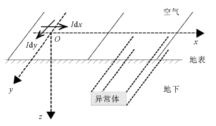
任何电磁问题都满足Maxwell方程组。FSM在实际应用中应尽量避开高压线等强烈的人文干扰。在FSM所满足的条件下,建立如图1所示的地质地球物理模型,,y轴平行构造走向,电性参数仅随x和z方向发生变化。将场源放置在坐标原点O,既可沿x轴也可以沿y轴。

图1

新窗口打开| 下载原图ZIP| 生成PPT

图1 二维地电模型与坐标系

Fig.1 2D geoelectrical model and coordinate system

假定圆频率为ω、谐变因子为eⁱ^ωt,在导电介质中忽略位移电流时,则谐变电磁场的基本微分方程为

(1)

\{\begin{array}{l} \nabla \times E = - i ω μ H, \\ \nabla \times H = σ E + J_{e} 。 \end{array}

式中:E和H分别为电场强度和磁场强度;J_e为源电流密度;μ、σ分别为介质的磁导率和电导率;t为时间变量;i为虚数单位,i²=-1。

将方程组(1)在直角坐标系中展开,并作傅立叶变换,则可得到波数域的6个偏微分方程^[19]:

(2)

\{\begin{array}{l} i k_{y} {\hat{E}}_{z} - \frac{\partial {\hat{E}}_{y}}{\partial z} = - i ω μ {\hat{H}}_{x}, \\ \frac{\partial {\hat{E}}_{x}}{\partial z} - \frac{\partial {\hat{E}}_{z}}{\partial x} = - i ω μ {\hat{H}}_{y}, \\ \frac{\partial {\hat{E}}_{y}}{\partial x} - i k_{y} {\hat{E}}_{x} = - i ω μ {\hat{H}}_{z}, \\ i k_{y} {\hat{H}}_{z} - \frac{\partial {\hat{H}}_{y}}{\partial z} = σ_{x x} {\hat{E}}_{x} + σ_{x y} {\hat{E}}_{y} + σ_{x z} {\hat{E}}_{z} + {\dot{J}}_{e x}, \\ \frac{\partial {\hat{H}}_{x}}{\partial z} - \frac{\partial {\hat{H}}_{z}}{\partial x} = σ_{y x} {\hat{E}}_{x} + σ_{y y} {\hat{E}}_{y} + σ_{y z} {\hat{E}}_{z} + {\dot{J}}_{e y}, \\ \frac{\partial {\hat{H}}_{y}}{\partial x} - i k_{y} {\hat{H}}_{x} = σ_{z x} {\hat{E}}_{x} + σ_{z y} {\hat{E}}_{y} + σ_{z z} {\hat{E}}_{z} + {\dot{J}}_{e z} 。 \end{array}

式中: $k_{y}$ 为波数;^代表波数域内的参数。

将式(2)的6个方程进行重组,形成只含有电场 ${\hat{E}}_{y} 和磁场 {\hat{H}}_{y}$ 的2个对偶方程:

(3)$\begin{array}{c} F \hat{E}_{y}+M G \frac{\partial \hat{E}_{y}}{\partial x}+M H \frac{\partial \hat{E}_{y}}{\partial z}-R\left[\left(\sigma_{x x}-\mathrm{i} \frac{k_{y}^{2}}{\omega \mu}\right) \frac{\partial^{2} \hat{E}_{y}}{\partial z^{2}}+\left(\sigma_{z z}-\mathrm{i} \frac{k_{y}^{2}}{\omega \mu}\right) \frac{\partial^{2} \hat{E}_{y}}{\partial x^{2}}\right]+ \\ R\left[\sigma_{z x} \frac{\partial}{\partial z}\left(\frac{\partial \hat{E}_{y}}{\partial x}\right)+\sigma_{x z} \frac{\partial}{\partial x}\left(\frac{\partial \hat{E}_{y}}{\partial z}\right)\right]+\frac{1}{\mathrm{i} \omega \mu}\left(\frac{\partial^{2} \hat{E}_{y}}{\partial z^{2}}+\frac{\partial^{2} \hat{E}_{y}}{\partial x^{2}}\right)-\frac{P}{B} \frac{\partial \hat{H}_{y}}{\partial x}-\frac{Q}{B} \frac{\partial \hat{H}_{y}}{\partial z}+ \\ M\left(\sigma_{z x} \frac{\partial^{2} \hat{H}_{y}}{\partial z^{2}}-\sigma_{x z} \frac{\partial^{2} \hat{H}_{y}}{\partial x^{2}}\right)+M\left[\left(\sigma_{x x}-\frac{\mathrm{i} k_{y}^{2}}{\omega \mu}\right) \frac{\partial}{\partial z}\left(\frac{\partial \hat{H}_{y}}{\partial x}\right)-\left(\sigma_{z z}-\frac{\mathrm{i} k_{y}^{2}}{\omega \mu}\right) \frac{\partial}{\partial x}\left(\frac{\partial \hat{H}_{y}}{\partial z}\right)\right]= \\ \hat{J}_{\mathrm{e} y}+\frac{Q}{B} \hat{J}_{\mathrm{e} x}-M\left(\sigma_{z x} \frac{\partial \hat{J}_{\mathrm{e} x}}{\partial z}-\sigma_{z z} \frac{\partial \hat{J}_{\mathrm{e} x}}{\partial x}+\frac{\mathrm{i} k_{y}^{2}}{\omega \mu} \frac{\partial \hat{J}_{\mathrm{e} x}}{\partial x}\right), \end{array}$

(4)$\begin{array}{c} -\frac{A}{B} \frac{\partial \hat{E}_{y}}{\partial x}-\frac{C}{B} \frac{\partial \hat{E}_{y}}{\partial z}+M \sigma_{z x} \frac{\partial}{\partial x}\left(\frac{\partial \hat{E}_{y}}{\partial x}\right)-M \sigma_{x z} \frac{\partial}{\partial z}\left(\frac{\partial \hat{E}_{y}}{\partial z}\right)-M\left(\sigma_{x x}-\frac{\mathrm{i} k_{y}^{2}}{\omega \mu}\right) \frac{\partial}{\partial x}\left(\frac{\partial \hat{E}_{y}}{\partial z}\right)+ \\ M\left(\sigma_{z z}-\frac{\mathrm{i} k_{y}^{2}}{\omega \mu}\right) \frac{\partial}{\partial z}\left(\frac{\partial \hat{E}_{y}}{\partial x}\right)+\frac{\sigma_{z x}}{B} \frac{\partial}{\partial x}\left(\frac{\partial \hat{H}_{y}}{\partial z}\right)+\frac{\sigma_{x z}}{B} \frac{\partial}{\partial z}\left(\frac{\partial \hat{H}_{y}}{\partial x}\right)+\frac{1}{B}\left(\sigma_{x x}-\frac{\mathrm{i} k_{y}^{2}}{\omega \mu}\right) \frac{\partial}{\partial x}\left(\frac{\partial \hat{H}_{y}}{\partial x}\right)+ \\ \frac{1}{B}\left(\sigma_{z z}-\frac{\mathrm{i} k_{y}^{2}}{\omega \mu}\right) \frac{\partial}{\partial z}\left(\frac{\partial \hat{H}_{y}}{\partial z}\right)+\mathrm{i} \omega \mu \hat{H}_{y}=-\frac{\sigma_{z x}}{B} \frac{\partial \hat{J}_{\mathrm{e} x}}{\partial x}-\frac{1}{B}\left(\sigma_{z z}-\frac{\mathrm{i} k_{y}^{2}}{\omega \mu}\right) \frac{\partial \hat{J}_{\mathrm{e} x}}{\partial z} ; \end{array}$

式中的中间变量计算式分别为

$A = σ_{z y} σ_{x x} - σ_{x y} σ_{z x} - σ_{z y} \cdot \frac{i k_{y}^{2}}{ω μ}$ ,

$B = σ_{x z} σ_{z x} - σ_{x x} σ_{z z} + (σ_{x x} + σ_{z z}) \frac{i k_{y}^{2}}{ω μ} + \frac{k_{y}^{4}}{ω^{2} μ^{2}}$ ,

$C = σ_{z y} σ_{x z} + σ_{x y} \frac{i k_{y}^{2}}{ω μ} - σ_{x y} σ_{z z}$ ,

$M = \frac{k_{y}}{ω μ B}$ ,

$F = \frac{C}{B} σ_{y x} - σ_{y y} - \frac{A}{B} σ_{y z}$ ,

$G = C - σ_{y x} σ_{z z} + σ_{z x} σ_{y z} + \frac{i k_{y}^{2} σ_{y x}}{ω μ}$ ,

$H = - A + σ_{x z} σ_{y x} - σ_{x x} σ_{y z} + \frac{i k_{y}^{2} σ_{y z}}{ω μ}$ ,

$P = σ_{y x} σ_{x z} - σ_{x x} σ_{y z} + \frac{i k_{y}^{2} σ_{y z}}{ω μ}$ ,

$Q = σ_{y x} σ_{z z} - σ_{z x} σ_{y z} - \frac{i k_{y}^{2} σ_{y x}}{ω μ}$ ,

$R = \frac{k_{y}^{2}}{ω^{2} μ^{2} B}$ 。

式(3)和式(4)即为CSAMT正演问题所要求解的偏微分方程组,解该方程组能够得到电场 ${\hat{E}}_{y}$ 以及磁场 ${\hat{H}}_{y}$ 2个分量的值,其他的4个分量 ${\hat{E}}_{x}$ 、 ${\hat{E}}_{z}$ 、 ${\hat{H}}_{x}$ 和 ${\hat{H}}_{z}$ 可以通过解波数域内的麦克斯韦方程组得到。例如,分量 ${\hat{E}}_{x}$ 的具体求解形式为

(5)$\hat{E}_{x}=-\frac{C}{B} \hat{E}_{y}+\frac{k_{y}}{\omega \mu B}\left(\sigma_{z z}-\frac{\mathrm{i} k_{y}^{2}}{\omega \mu}\right) \frac{\partial \hat{E}_{y}}{\partial x}-\frac{k_{y} \sigma_{x z}}{\omega \mu B} \frac{\partial \hat{E}_{y}}{\partial z}+\frac{\sigma_{x z}}{B} \frac{\partial \hat{H}_{y}}{\partial x}+\frac{1}{B}\left(\sigma_{z z}-\frac{\mathrm{i} k_{y}^{2}}{\omega \mu}\right) \frac{\partial \hat{H}_{y}}{\partial z}+\frac{1}{B}\left(\sigma_{z z}-\frac{\mathrm{i} k_{y}^{2}}{\omega \mu}\right) \hat{J}_{\mathrm{ex}} 。$

其余3个分量 ${\hat{E}}_{z}$ 、 ${\hat{H}}_{x}$ 和 ${\hat{H}}_{z}$ 的具体计算式可参考文献[19]。

1.2 波数域电磁场二维有限单元法^[19]

用有限单元法求解泛函极值问题时,要将研究的区域剖分为有限个数的单元,各单元内场的分布由各单元节点处的场值来近似表示,由此将求泛函极值问题转化为求多元函数的极值问题。

令二维有限单元法的研究区域为Ω,其外围边界为∂Ω,有限单元法的残差R^E、R^H分别为式(3)、(4)的左右两边之差。根据Galerkin有限单元法,加权余量满足以下关系式

(6)

\overset{m}{\sum_{e = i}} \int \int N_{i} R^{E} d x d z = 0,

式中:e代表单元号;m为单元总数;N_i是第i个节点的插值函数。

由格林公式:

(7)

\iint ϕ \frac{\partial φ}{\partial x} d x d z = - \iint \frac{\partial ϕ}{\partial x} φ d x d z + \oint ϕ φ n_{x} d l,

可得单元内波数域场 ${\hat{E}}_{y}$ 和 ${\hat{H}}_{y}$ 函数:

(8)

\{\begin{array}{l} {\hat{E}}_{y Ω} = \sum_{k} N_{k} {\hat{E}}_{y k}, \\ {\hat{H}}_{y Ω} = \sum_{k} N_{k} {\hat{H}}_{y k} 。 \end{array}

式中N_k是第k个节点的二次插值函数。

引入双线性插值,运用Galerkin法可得到正演最终所要求解的有限元方程组为

(9)$\begin{array}{c} \sum_{e=1}^{m} \iint_{\Omega}\left\{-N_{i}^{e} N_{j} F \hat{E}_{y}+M G \frac{\partial N_{i}^{e}}{\partial x} N_{j} \hat{E}_{y}+M H \frac{\partial N_{i}^{e}}{\partial z} N_{j} \hat{E}_{y}-R\left(\sigma_{x x}-\frac{\mathrm{i} k_{y}^{2}}{\omega \mu}\right) \frac{\partial N_{i}^{e}}{\partial z} \frac{\partial N_{j}}{\partial z} \hat{E}_{y}-\right. \\ R\left(\sigma_{z z}-\frac{\mathrm{i} k_{y}^{2}}{\omega \mu}\right) \frac{\partial N_{i}^{e}}{\partial x} \frac{\partial N_{j}}{\partial x} \hat{E}_{y}+R \sigma_{z x} \frac{\partial N_{i}^{e}}{\partial z} \frac{\partial N_{j}}{\partial x} \hat{E}_{y}+R \sigma_{x z} \frac{\partial N_{i}^{e}}{\partial x} \frac{\partial N_{j}}{\partial z} \hat{E}_{y}+\frac{1}{\mathrm{i} \omega \mu}\left(\frac{\partial N_{i}^{e}}{\partial z} \frac{\partial N_{j}}{\partial z} \hat{E}_{y}+\right. \\ \left.\frac{\partial N_{i}^{e}}{\partial x} \frac{\partial N_{j}}{\partial x} \hat{E}_{y}\right)-\frac{P}{B} \frac{\partial N_{i}^{e}}{\partial x} N_{j} \hat{H}_{y}-\frac{Q}{B} \frac{\partial N_{i}^{e}}{\partial z} N_{j} \hat{H}_{y}+M\left(\sigma_{z x} \frac{\partial N_{i}^{e}}{\partial z} \frac{\partial N_{j}}{\partial z} \hat{H}_{y}-\sigma_{x z} \frac{\partial N_{i}^{e}}{\partial x} \frac{\partial N_{j}}{\partial x} \hat{H}_{y}\right)+ \\ \left.M\left[\left(\sigma_{x x}-\frac{\mathrm{i} k_{y}^{2}}{\omega \mu}\right) \frac{\partial N_{i}^{e}}{\partial z} \frac{\partial N_{j}}{\partial x} \hat{H}_{y}-\left(\sigma_{z z}-\frac{\mathrm{i} k_{y}^{2}}{\omega \mu}\right) \frac{\partial N_{i}^{e}}{\partial x} \frac{\partial N_{j}}{\partial z} \hat{H}_{y}\right]\right\} \mathrm{d} x \mathrm{~d} z= \\ \sum_{e=1}^{m} \iint_{\Omega}\left\{N_{i}^{e} \hat{J}_{\mathrm{e} y}+\frac{Q}{B} N_{i}^{e} \hat{J}_{\mathrm{e} x}-M \sigma_{z x} \frac{\partial N_{i}^{e}}{\partial z} \hat{J}_{\mathrm{e} x}+M \sigma_{z z} \frac{\partial N_{i}^{e}}{\partial x} \hat{J}_{\mathrm{e} x}-\frac{\mathrm{i} k_{y}^{2} M}{\omega \mu} \frac{\partial N_{i}^{e}}{\partial x} \hat{J}_{\mathrm{e} x}\right\} \mathrm{d} x \mathrm{~d} z, \end{array}$

(10)$\begin{array}{c} \sum_{e=1}^{m} \iint_{\Omega}\left[-\frac{A}{B} \frac{\partial N_{i}^{e}}{\partial x} N_{j} \hat{E}_{y}-\frac{C}{B} \frac{\partial N_{i}^{e}}{\partial z} N_{j} \hat{E}_{y}+M \sigma_{z x} \frac{\partial N_{i}^{e}}{\partial x} \frac{\partial N_{j}}{\partial x} \hat{E}_{y}-M \sigma_{x z} \frac{\partial N_{i}^{e}}{\partial z} \frac{\partial N_{j}}{\partial z} \hat{E}_{y}-\right. \\ M\left(\sigma_{x x}-\frac{i k_{y}^{2}}{\omega \mu}\right) \frac{\partial N_{i}^{e}}{\partial x} \frac{\partial N_{j}}{\partial z} \hat{E}_{y}+M\left(\sigma_{z z}-\frac{\mathrm{i} k_{y}^{2}}{\omega \mu}\right) \frac{\partial N_{i}^{e}}{\partial z} \frac{\partial N_{j}}{\partial x} \hat{E}_{y}+\frac{\sigma_{z x}}{B} \frac{\partial N_{i}^{e}}{\partial x} \frac{\partial N_{j}}{\partial z} \hat{H}_{y}+\frac{\sigma_{x z}}{B} \frac{\partial N_{i}^{e}}{\partial z} \frac{\partial N_{j}}{\partial x} \hat{H}_{y}+ \\ \left.\frac{1}{B}\left(\sigma_{x x}-\frac{\mathrm{i} k_{y}^{2}}{\omega \mu}\right) \frac{\partial N_{i}^{e}}{\partial x} \frac{\partial N_{j}}{\partial x} \hat{H}_{y}+\frac{1}{B}\left(\sigma_{z z}-\frac{\mathrm{i} k_{y}^{2}}{\omega \mu}\right) \frac{\partial N_{i}^{e}}{\partial z} \frac{\partial N_{j}}{\partial z} \hat{H}_{y}-\mathrm{i} \omega \mu N_{i}^{e} N_{j} \hat{H}_{y}\right] \mathrm{d} x \mathrm{~d} z= \\ \sum_{e=1}^{m} \iint_{\Omega}\left[-\frac{\sigma_{z x}}{B} \frac{\partial N_{i}^{e}}{\partial x} \hat{J}_{\mathrm{e} x}-\frac{1}{B}\left(\sigma_{z z}-\frac{\mathrm{i} k_{y}^{2}}{\omega \mu}\right) \frac{\partial N_{i}^{e}}{\partial z} \hat{J}_{\mathrm{e} x}\right] \mathrm{d} x \mathrm{~d} z_{\circ} \end{array}$

式中: $N_{e}$ 表示剖分的总单元数; $N_{i}^{e}$ 表示第e个单元中第i个节点的插值函数。

由式(9)、(10)可求得各个节点处波数域的电磁场 ${\hat{E}}_{y} 、 {\hat{H}}_{y}$ ,再由式(5)求 ${\hat{E}}_{x}$ ,式中各个节点处 ${\hat{E}}_{y} 、 {\hat{H}}_{y}$ 的方向偏导数可由插值获得。采用Galerkin加权余量法建立有限单元方程,即可实现波数域有限单元法计算。

2 天然电场选频法的模拟计算与分析

利用上述二维有限单元法模拟理论,即可对FSM的二维地质地球物理模型开展模拟计算。由于FSM一般只观测沿测线方向的地表水平电场分量,即沿x方向的分量E_x,所以,下面仅对TM极化模式进行讨论。

设置2个模型进行模拟计算。模型的场源长度为200 m,发射电流为100 A,计算频率f 为10¹、10^1.25、10^1.5、10^1.75、10² Hz,场源到测线的垂直距离为6.6 km。采用矩形网格对模型进行剖分,剖分原则为:对异常体赋存区域以均匀网格剖分,对无异常体的网格外延区域,网格步长按大于1的倍数递增。这样,可在保证计算精度的情况下减少网格剖分数,节省计算时间。

2.1 模型1

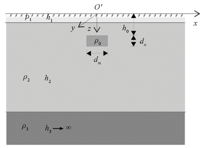
模型1如图2所示。假设一个三层水平介质模型,从地表往下的岩性分别为细粒松散沉积物、白云质灰岩和花岗岩,电阻率分别为ρ₁=350 Ω·m、ρ₂=1 500 Ω·m、ρ₃=5 500 Ω·m,覆盖层厚度h₁=80 m、h₂=1 000 m;在白云质灰岩中存在一个被地下水充填的低阻岩溶异常体,假定其电阻率 $ρ_{0}$ =40 Ω·m,大小为160 m×80 m,即d_m=160 m、d_n=80 m,其顶部埋深h₀=200 m。根据上述模拟参数可知,图2中的点O'距离图1中的坐标原点O的距离即为6.6 km。

图2

新窗口打开| 下载原图ZIP| 生成PPT

图2 层状介质中的异常体模型1

Fig.2 A abnormal body in layered half space of model 1

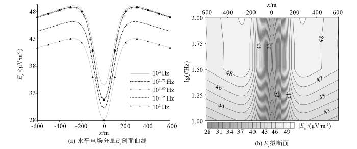
图3为模型1的5个频率模拟结果。由水平电场分量 $E_{x}$ 的剖面结果(图3a)可见, $E_{x}$ 的剖面曲线在x=0处出现极小值,且 $E_{x}$ 曲线随着频率的升高而整体向上抬升,总体形态不变,相对异常大小变化不明显;其中,10^1.50Hz与10^1.75Hz二者的剖面曲线差异较小,在图中几乎重合在一起。在 $E_{x}$ 拟断面图中(图3b), $E_{x}$ 值随频率的降低而减小,且等值线在低阻体正上方(x=0 m)附近出现向上拉伸现象,即“挂面条”现象,等值线在x=0 m附近较密集,梯度变化较大。

图3

新窗口打开| 下载原图ZIP| 生成PPT

图3 模型1的模拟计算结果

Fig.3 Simulation calculation results of model 1

图3的特征就是频率域电磁法静态效应的典型表现。同时,图3a的剖面曲线形态与FSM在地下水勘探中的实测曲线形态是基本相同的,FSM正是利用剖面曲线的低值点来确定成井位置^[12]。

2.2 模型2

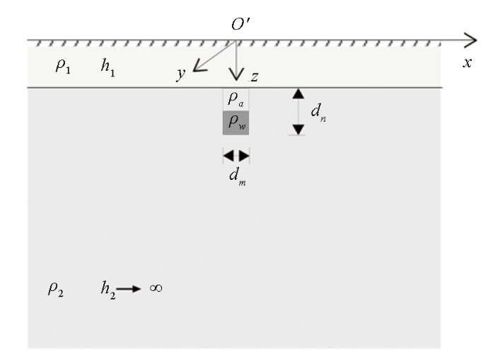
如图4所示模型2,假设一个二层水平介质,岩性分别为第四系覆盖层和白云岩,电阻率分别为ρ₁=140 Ω·m、 $ρ_{2} = 2$ 000 Ω·m,覆盖层的厚度 $h_{1} = 20$ m。基岩中有一矩形异常体,其顶部埋深 $h_{0} = h_{1} =$ 20 m,即顶面与岩性分界面齐平,宽度 $d_{m} =$ 10 m、高度 $d_{n} =$ 20 m;假定异常体为泥质半充填状态,即充填高度为10 m,上部10 m为空气。令泥质的电阻率ρ_w=60 Ω·m,空气的电阻率为 $ρ_{a} =$ 60 000 Ω·m。

图4

新窗口打开| 下载原图ZIP| 生成PPT

图4 层状介质中的异常体模型2

Fig.4 A abnormal body in layered half space of model 2

图5为模型2的模拟计算结果。图5a中的水平电场分量 $E_{x}$ 剖面曲线特征与图3a中的剖面曲线特征相似,曲线随着频率的升高而整体向上平移,相对异常大小变化也不明显,但10^1.75Hz与10²Hz二者的剖面曲线差异较小。图5b中, $E_{x}$ 拟断面图的总体特征也与图3b相同,在x=0 m附近等值线总体向上拉伸,出现比图3b 宽度窄一些的“挂面条”现象,这是由于模型2中异常体的宽度小于模型1的异常体宽度。

图5

新窗口打开| 下载原图ZIP| 生成PPT

图5 模型2的模拟计算结果

Fig.5 Simulation calculation results of model 2

由上述两个模型的模拟计算可知,由于近地表附近低阻异常体的存在,正演获得的水平电场分量 $E_{x}$ 的剖面曲线与野外FSM实测的电位差曲线形态特征相同,说明用上述正演理论模拟FSM的剖面曲线是可行的。同时,随着频率的变化, $E_{x}$ 剖面曲线和拟断面图呈现明显的静态效应现象,正是由于电场分量的这种静态偏移导致了电磁法勘探中视电阻率曲线 $ρ_{s}$ 出现静态效应。除静态偏移外, $E_{x}$ 剖面曲线随频率的升高整体向上抬升,也可能是由于随着频率的增大,勘探深度减小,浅部介质的信号增强所致;反之,随着频率的减小,勘探深度增大,深部介质在地表感应出的电场减弱,致使 $E_{x}$ 随着频率的减小而减小。

3 FSM实践应用

由以上正演分析可知:FSM实测剖面上的低电位曲线是由于近地表低阻体的存在所致,随着观测频率的增大,多条剖面曲线会呈现明显的静态效应现象;可见FSM是利用了频率域电磁法的静态效应现象来探测浅部地质体。下面进一步用实例来加以说明。

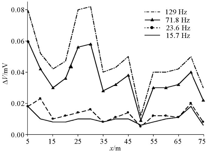
图6为MFE型选频仪在四川古叙煤田官文煤矿的勘探成果^[12],MN电极距为10 m,点距5 m,图中曲线旁的频率值为探测频率。在该测线平距50 m、埋深约80 m处存在充水岩溶。由图6可以看出,在低阻异常体的对应位置上出现了明显的低电位异常,曲线整体随着频率的增大出现向上抬升,这与前文的正演结果基本一致。

图6

新窗口打开| 下载原图ZIP| 生成PPT

图6 选频法在充水岩溶上的探测成果^[12]

Fig.6 Exploration results of FSM in water filled karst^[12]

在FSM的应用初期,仅测量一个或几个频率的剖面曲线,这大大限制了人们对其异常成因的认识。随着电子技术的发展和仪器智能化水平的提高,目前仪器的观测频率数已经达到几十,如TC150型智能化选频仪。

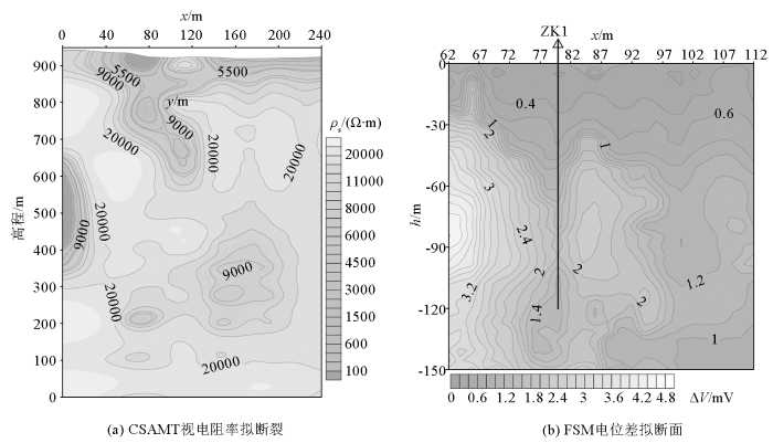
图7为鸳鸯草场地下水物探勘探成果。鸳鸯草场位于福建省柘荣县东源乡鸳鸯头村,距离县城18 km,海拔高程980~1 110 m,面积近万亩,为福建省最大的天然草场。该区域严重缺水,地表第四系以下为紫色、灰白色凝灰质砂砾岩、砂岩夹粉砂质泥岩。图7a为CSAMT的视电阻率拟断面,测量点距为20 m,图中可见,在剖面80 m附近的近地表出现向下延伸的低阻异常带,即存在静态效应。在以往的频率域电磁法勘探中,大多关注的是深部地质体,这种浅部的静态效应常常会被当作干扰予以压制或消除。在此,根据前面的正演分析结果,推测该剖面80 m附近的近地表存在地下水等低阻异常体,因此,进一步采用选频法对该浅部低阻异常体开展综合探测。选用TC150型智能化选频仪,工作频率33个,范围在100~5 000 Hz,点距为2 m,MN为10 m。图7b为选频法的电位差ΔV拟断面,其纵坐标视深度h是由电磁波的趋肤深度和经验系数反演获得的。由图7b可见,ΔV等值线在剖面80 m附近存在明显向下延伸的低电位异常带,即“挂面条”现象,这进一步验证了CSAMT静态效应异常的可靠性。在该剖面80 m处布置钻孔ZK1,钻井深度120 m,出水量为115 t/d。

图7

新窗口打开| 下载原图ZIP| 生成PPT

图7 鸳鸯草场地下水勘探成果

Fig.7 Map of groundwater exploration results in Yuanyang meadow

由上述应用实例可见,选频法(FSM)剖面曲线的低电位异常主要是由频率域电磁法的静态效应所致,其拟断面图中的“挂面条”现象也进一步验证了静态效应的存在;同时,FSM的应用实例说明,电磁法的静态效应现象是可以利用的,可将其用于浅部地质体的勘探。

4 结论

1)根据有限单元法的选频法(FSM)二维模拟研究可知,当近地表存在导电性异常体时,地表沿测线方向的水平电场分量 $E_{x}$ 剖面曲线会在低阻体正上方出现明显的低电位异常,这指明了近地表低阻体的存在及其水平投影位置。当观测频率增多时, $E_{x}$ 的剖面曲线随频率的增大而整体向上偏移,也就是频率域电磁法的静态偏移现象;而 $E_{x}$ 的拟断面图则出现“挂面条”现象,其等值线拉伸方向向上,这也正是静态效应在拟断面图中的典型表现。

2)FSM的实践应用成果及其与CSAMT在鸳鸯草场的实践对比结果表明,FSM的异常起因主要是由电磁法的静态效应所致;FSM在地下水勘探中的成功实例也说明,利用频率域电磁法的静态效应现象可以寻找浅部近地表导电性异常体。所以,今后也可利用MT、AMT和CSAMT等方法的静态效应现象来探测近地表的电性异常体,利用静态效应进行勘探则可称之为静态效应法。

尽管根据CSAMT的静态效应现象可较完美地解释FSM的剖面异常成因,但根据笔者的进一步试算可知,静态效应不能圆满解释FSM测深法的异常起因,同时也无法对FSM的动态效应现象做出合理解释,这些问题都有待今后进一步研究。

致谢

衷心感谢薛国强教授在本文撰写过程中给予的耐心指导和宝贵建议!感谢周印明博士在模拟计算方面提供的帮助!

参考文献

原文顺序

文献年度倒序

文中引用次数倒序

被引期刊影响因子

[1]

底青云, 朱日祥, 薛国强, 等.

我国深地资源电磁探测新技术研究进展

[J]. 地球物理学报, 2019, 62(6):2128-2138.

[本文引用: 1]

Q Y

, Zhu

R X

, Xue

G Q

, et al.

New development of the electromagnetic (EM) methods for deep exploration

[J]. Chinese Journal of Geophysics, 2019, 62(6):2128-2138.

[本文引用: 1]

[2]

Zonge

K L

Comparison of time,frequency and phase measurement in IP

[J]. Geophysical Prospecting, 1972, 20:626-648.

DOI:10.1111/gpr.1972.20.issue-3 URL [本文引用: 1]

[3]

Jones

A G

Static shift of magnetotelluric data and its removal in a sedimentary basin environment

[J]. Geophysics, 1988, 53(7):967-978.

DOI:10.1190/1.1442533 URL [本文引用: 1]

Previous modeling investigations of the static shift of magnetotelluric (MT) apparent resistivity curves have limited appeal in that the electric fields used were point measurements, whereas field observations are of voltage differences. Thus, inhomogeneities of dimension of the order of the electrode line length could not be investigated. In this paper, by using a modeling algorithm that derives point voltages rather than point electric fields, I consider the effect on the MT responses of local near‐surface distorting structures, which are both outside of, and inside, the telluric electrode array. I show that static‐shift effects are of larger spatial size but of less magnitude than would be expected from conventional modeling. Also, the field observation that static shift affects only the apparent resistivity curve but not the phase response can be replicated by the voltage difference modeling. If there exists within the earth a layer whose variation in electrical resistivity along the profile can be treated in a parametric fashion, then static shift of the apparent resistivity curves can be corrected. Deriving the modal value from a sufficient number of observations for the layer resistivity is the most useful approach.

[4]

Kaufman

A A

Reduction of the geological noise in magnetotelluric sounding

[J]. Geoexploration, 1988, 25:145-161.

DOI:10.1016/0016-7142(88)90010-5 URL [本文引用: 1]

[5]

Zonge

K L

, Hughes

L J

. Controlled source audio-frequency magnetotellurics[M]// Nabighian M N. Electromagnetic Methods: Theory and Practice, Society of Exploration Geophysicists, 1988.

[本文引用: 1]

[6]

Andrieux

, Wightman

W E

The so-called static corrections in magnetotelluric measurements

[C]// 54^th Ann. Mtg., Soc. Expl. Geophys., Expanded Abstracts, 1984:43-44.

[本文引用: 1]

[7]

Sternberg

B K

, Washburne

J C

, Pellerin

Correction for the static shift in magnetotellurics using transient electromagnetic soundings

[J]. Geophysics, 1988, 53:1459-1468.

DOI:10.1190/1.1442426 URL [本文引用: 1]

Shallow inhomogeneities can lead to severe problems in the interpretation of magnetotelluric (MT) data by shifting the MT apparent resistivity sounding curve by a scale factor, which is independent of frequency on the standard log‐apparent‐resistivity versus log‐frequency display. The amount of parallel shift, commonly referred to as the MT static shift, can not be determined directly from conventionally recorded MT data at a single site. One method for measuring the static shift is a controlled‐source measurement of the magnetic field. Unlike the electric field, the magnetic field is relatively unaffected by surface inhomogeneities. The controlled‐source sounding (which may be a relatively shallow sounding made with lightweight equipment) can be combined with a deep MT sounding to obtain a complete, undistorted model of the earth. Inversions of the static shift‐corrected MT data provide a much closer match to well‐log resistivities than do inversions of the uncorrected data. The particular controlled‐source magnetic‐field sounding which we used was a central‐induction Transient ElectroMagnetic (TEM) sounding. Correction for the static shift in the MT data was made by jointly inverting the MT data and the TEM data. A parameter which allowed vertical shifts in the MT apparent resistivity curves was included in the computer inversion to account for static shifts. A simple graphical comparison between the MT apparent resistivities and the TEM apparent resistivities produced essentially the same estimate of the static shift (within 0.1 decade) as the joint computer inversion. Central‐induction TEM measurements were made adjacent to over 100 MT sites in central Oregon. The complete data base of over 100 sites showed an average static shift between 0 and 0.2 decade. However, in the rougher topography and more complex structure of the Cascade Mountain Range, the majority of the sites had static shifts of the order of 0.3 to 0.4 decade. The static shifts in this area are probably due to a combination of topography and surficial inhomogeneities. The TEM apparent resistivity (which is used to estimate the unshifted MT apparent resistivity) does not necessarily agree with either the transverse electric (TE) or the transverse magnetic (TM) MT polarization. TEM apparent resistivity may occur between the two, or may agree with one of the two polarizations, or may lie outside the MT polarizations.

[8]

陈清礼, 张翔, 胡文宝.

南方碳酸盐岩区大地电磁测深曲线静态偏移校正

[J]. 江汉石油学院学报, 1999, 21(3):30-32.

[本文引用: 1]

Chen

Q L

, Zhang

, Hu

W B

Static migration correction of magnetotelluric sounding curve in carbonate area of South China

[J]. Journal of Jianghan Petroleum Institute, 1999, 21(3):30-32.

[本文引用: 1]

[9]

杨生, 鲍光淑, 李爱勇.

MT法中静态效应及阻抗张量静态校正法

[J]. 中南工业大学学报, 2002, 33(1):8-13.

[本文引用: 1]

Yang

, Bao

G S

, Li

A Y

The static migration to MT data and the impedance tensor static correction method

[J]. Journal of CentralSouth University of Technology, 2002, 33(1):8-13.

[本文引用: 1]

[10]

邱卫忠, 闫述, 薛国强, 等.

CSAMT的各分量在山地精细勘探中的作用

[J]. 地球物理学进展, 2011, 26(2):664-668.

[本文引用: 1]

Qiu

W Z

, Yan

, Xue

G Q

, et al.

Action of CSAMT field components in mountainous fine prospecting

[J]. Progress in Geophysics, 2011, 26(2):664-668.

[本文引用: 1]

[11]

于生宝, 郑建波, 高明亮, 等.

基于小波变换模极大值法和阈值法的CSAMT静态校正

[J]. 地球物理学报, 2017, 60(1):360-368.

[本文引用: 1]

S B

, Zheng

J B

, Gao

M L

, et al.

CSAMT static correction method based on wavelet transform modulus maxima and thresholds

[J]. Chinese Journal of Geophysics, 2017, 60(1):360-368.

[本文引用: 1]

[12]

杨天春, 夏代林, 王齐仁, 等. 天然电场选频法理论研究与应用[M]. 长沙: 中南大学出版社, 2017.

[本文引用: 6]

Yang

T C

, Xia

D L

, Wang

Q R

, et al. Theoretical research and application of frequency selection method for telluric electricity field[M]. Changsha: Central South University Press, 2017.

[本文引用: 6]

[13]

杨杰

游散电流法在岩溶地区的试验成果及理论研究

[J]. 物探与化探, 1982, 6(1):41-54.

[本文引用: 1]

Yang

Experimental results and theoretical study of the stray current method in karst area

[J]. Geophysical and Geochemical Exploration, 1982, 6(1):41-54.

[本文引用: 1]

[14]

林君琴, 雷长声, 董启山.

天然低频电场法

[J]. 长春地质学院学报, 1983, 13(2):114-126.

[本文引用: 1]

Lin

J Q

, Lei

C S

, Dong

Q S

The natural low frequency electric field method

[J]. Journal of Jilin University, 1983, 13(2):114-126.

[本文引用: 1]

[15]

杨天春, 陈卓超, 梁竞, 等.

天然电场选频测深法在地下水勘探中的异常理论分析与实践应用

[J]. 地学前缘, 2020, 27(4):302-310.

DOI:10.13745/j.esf.sf.2020.6.34 [本文引用: 2]

选频法是音频大地电场法的进一步应用与发展。本文通过实践应用说明选频法在浅层地下水勘探中的有效性,并对选频法测深极距(MN)与地下水埋深之间的关系开展对比分析和初步理论研究。首先,采用水平交变电场、交变磁场共同作用下的均匀半空间中低阻导电球体简化地质地球物理模型,对选频法测深曲线开展正演计算;然后,对选频法在广西“十二五”农村饮水安全工程应用中的131口钻井出水量情况进行统计,并对其中98口钻井的钻探情况开展详细列表统计分析,对比研究测深曲线异常处MN极距大小与实际钻探出水深度之间的关系。理论分析与实践应用表明,选频法在浅层地下水勘探中效果明显,是一种确定浅层地下水井位的有效方法;同时,实践统计结果表明,选频法测深法异常曲线处MN极距的大小与实际钻探出水深度之间存在1∶1的近似关系,验证了理论模拟计算结果的正确性;另外,本文的研究成果表明,在浅层(<200 m)天然电磁法勘探中,天然电场观测值的大小除了与大地的电阻率、信号的频率有关外,还与电极距大小是相关的。

Yang

T C

, Chen

Z C

, Liang

, et al.

Theoretical analysis of sounding anomaly and field application of the natural electric field frequency selection sounding method in groundwater exploration

[J]. Earth Science Frontiers, 2020, 27(4):302-310.

DOI:10.13745/j.esf.sf.2020.6.34 [本文引用: 2]

The frequency selection method is a further development of the audio frequency telluric electricity field method. In this report, we illustrate the usefulness of the method in shallow groundwater exploration through field application examples. We studied the relationship between potential electrode spacing MN and groundwater depth and carried out preliminary theoretical analysis. Firstly, under the combined action of horizontal alternating electric and magnetic fields, we established a simplified geophysical model of low resistivity conductive sphere in homogeneous half space, and performed forward calculation on the sounding curve. We then recorded water yields of 131 rural drinking wells in Guangxi Province. In addition, we performed detailed tabular statistical analysis of 98 drilling wells, and compared the relationship between potential electrode spacing MN in abnormal sounding curve and actual drilling water depth. Theoretical analysis and field application show that the frequency selection method can be very useful in shallow groundwater exploration for determining shallow groundwater well location. At the same time, the tabular statistics show that there is 1∶1 approximation between the size of potential electrode spacing MN in the anomaly curve and actual drilling water depth, validating the theoretical simulation results. Moreover, we show that the observed value of telluric electric field is related not only to the Earth's resistivity and signal frequency, but also to the potential electrode spacing in a shallow (< 200 m) magnetotelluric exploration.

[16]

Yang

T C

, Gao

Q S

, Li

, et al.

New insights into the anomaly genesis of the frequency selection method:Supported by numerical modeling and case studies

[J]. Pure and Applied Geophysics, 2023. http://doi.org/10.1007/s00024-022-03220-8

URL [本文引用: 1]

[17]

Ren

, Kalscheuer

, Greenhalgh

, et al.

A goal-oriented adaptive finite-element approach for plane wave 3-D electromagnetic modeling

[J]. Geophysical Journal International, 2013, 194(2):700-718.

DOI:10.1093/gji/ggt154 URL [本文引用: 1]

[18]

杨天春, 张正发, 许德根, 等.

花岗岩地区浅部地下水井位的快速确定

[J]. 水文地质工程地质, 2017, 44(5):20-24,32.

[本文引用: 1]

Yang

T C

, Zhang

Z F

, Xu

D G

, et al.

Fast determination of shallow groundwater wells in a granite area

[J]. Hydrogeology & Engineering Geology, 2017, 44(5):20-24,32.

[本文引用: 1]

[19]

王汪汪

. 可控源音频大地电磁法二维各向异性正演研究[D]. 北京: 中国地质大学, 2017.

[本文引用: 3]

Wang

W W

. Controlled-source audio-frequency magnetotelluric two-dimensional modeling for arbitrary anisotropy structures[D]. Beijing: China University of Geosciences (Beijing), 2017.

[本文引用: 3]

我国深地资源电磁探测新技术研究进展

2019

... 在频率域电磁测深中,受浅层不均匀体和地形起伏的影响,电流流过不均匀体表面时会形成“积累电荷”,即地下电流密度分布出现畸变,致使地表观测的电场分量出现突然增强或减弱,测得的视电阻率曲线与正常曲线相比出现上下平移现象,这就是电磁法的静态效应^[1].特别是当电磁波的趋肤深度远大于不均匀体尺寸时,其影响就不可忽略.对于视电阻率拟断面图而言,静态效应一般表现为密集的直立等值线,纵向延伸很大,横向范围比较小,如实际资料中出现的所谓“挂面条”现象,大部分是静态位移效应所致. ...

我国深地资源电磁探测新技术研究进展

2019

Comparison of time,frequency and phase measurement in IP

1972

... 静态效应是频率域电磁法应用中无法避免的一种物理现象,它会引起资料解释成果出现偏差或错误,因此一般将其作为干扰进行压制和消除,以此提高深部信号的信噪比.如:Zonge^[2]在希尔伯特变换的基础上,导出振幅谱与相位谱之间的关系,根据静态效应不影响相位数据的原理,提出了相位校正法;Bostick针对消除大地电磁法(MT)中静态干扰而提出电磁阵列剖面法^[3];Kaufman^[4]提出了与EMAP原理相似的曲线拟合法;Zonge等^[5]采用曲线平移法压制静态效应;Andrieux、Sternberg等^[6-7]提出利用瞬变电磁法(TEM)消除静位移对MT曲线解释结果的影响.国内学者对静态偏移校正也开展了许多研究工作:陈清礼等^[8]利用地表出露地层的电阻率来标定视电阻率曲线的首支,以此确定静态偏移量,并利用该偏移量去改正MT的视电阻率曲线;杨生等^[9]提出了对阻抗张量或实测的电场分量实施静态校正的方法;邱卫忠等^[10]对可控源音频大地电磁法(CSAMT)的单分量电场进行了研究;于生宝等^[11]提出了基于小波变换模极大值法和阈值法的CSAMT静态校正. ...

Static shift of magnetotelluric data and its removal in a sedimentary basin environment

1988

Reduction of the geological noise in magnetotelluric sounding

1988

The so-called static corrections in magnetotelluric measurements

1984

Correction for the static shift in magnetotellurics using transient electromagnetic soundings

1988

南方碳酸盐岩区大地电磁测深曲线静态偏移校正

1999

南方碳酸盐岩区大地电磁测深曲线静态偏移校正

1999

MT法中静态效应及阻抗张量静态校正法

2002

MT法中静态效应及阻抗张量静态校正法

2002

CSAMT的各分量在山地精细勘探中的作用

2011

CSAMT的各分量在山地精细勘探中的作用

2011

基于小波变换模极大值法和阈值法的CSAMT静态校正

2017

基于小波变换模极大值法和阈值法的CSAMT静态校正

2017

... 天然电场选频法(简称选频法,FSM)是以往中国学者在文献中提到的电脉冲自然电场法等众多方法的总称^[12],它是由中国学者于20世纪80年代提出来的,通过在地面上测量天然交变电磁场产生的一个或几个不同频率的电场水平分量的变化规律,来研究地下地电断面的电性变化.以往指针式仪器的工作频率一般为15~1 500 Hz,目前智能化仪器大多为10~5 000 Hz;在开展剖面法观测时,MN的极距大小一般取10 m或20 m.过去人们对FSM的研究主要集中在仪器研制和实践应用两方面,而对其理论研究甚少.杨杰、林君琴等^[13-14]曾分别以不同的场源观点对FSM开展过理论探讨;杨天春等^[12,15]推导并计算了简单二维地质地球物理模型的FSM异常,并对三维电磁场共同作用下球体的异常进行过正演模拟;近期,Yang T C等^[16]又基于MT理论对FSM的剖面异常开展了理论分析. ...

... [12,15]推导并计算了简单二维地质地球物理模型的FSM异常,并对三维电磁场共同作用下球体的异常进行过正演模拟;近期,Yang T C等^[16]又基于MT理论对FSM的剖面异常开展了理论分析. ...

... 图3的特征就是频率域电磁法静态效应的典型表现.同时,图3a的剖面曲线形态与FSM在地下水勘探中的实测曲线形态是基本相同的,FSM正是利用剖面曲线的低值点来确定成井位置^[12]. ...

... 图6为MFE型选频仪在四川古叙煤田官文煤矿的勘探成果^[12],MN电极距为10 m,点距5 m,图中曲线旁的频率值为探测频率.在该测线平距50 m、埋深约80 m处存在充水岩溶.由图6可以看出,在低阻异常体的对应位置上出现了明显的低电位异常,曲线整体随着频率的增大出现向上抬升,这与前文的正演结果基本一致. ...

... [12] Exploration results of FSM in water filled karst<sup>[<xref ref-type="bibr" rid="b12">12</xref>]</sup>

Fig.6

在FSM的应用初期,仅测量一个或几个频率的剖面曲线,这大大限制了人们对其异常成因的认识.随着电子技术的发展和仪器智能化水平的提高,目前仪器的观测频率数已经达到几十,如TC150型智能化选频仪. ...

... [12]Fig.6

2017

... [12] Exploration results of FSM in water filled karst<sup>[<xref ref-type="bibr" rid="b12">12</xref>]</sup>

Fig.6

... [12]Fig.6

游散电流法在岩溶地区的试验成果及理论研究

1982

游散电流法在岩溶地区的试验成果及理论研究

1982

天然低频电场法

1983

天然低频电场法

1983

天然电场选频测深法在地下水勘探中的异常理论分析与实践应用

2020

... 根据以往的应用可知,相对于MT或AMT而言,选频法(FSM)的勘探深度一般比较浅,大多在200 m之内^[15,18],所以,其一次场场源除了与MT一样有地球之外的场源外,地表人文活动所产生的干扰信号也会成为主要场源.由此,可用CSAMT理论来近似模拟FSM的信号. ...

天然电场选频测深法在地下水勘探中的异常理论分析与实践应用

2020

New insights into the anomaly genesis of the frequency selection method:Supported by numerical modeling and case studies

2023

A goal-oriented adaptive finite-element approach for plane wave 3-D electromagnetic modeling

2013

... 电磁法的正演方法主要有积分方程法、有限差分法和有限元法等,其中有限单元法在电磁法正演模拟方面有其自身的优势^[17],成熟的理论与方法已使其成为研究电磁法问题的重要手段之一. ...

花岗岩地区浅部地下水井位的快速确定

2017

花岗岩地区浅部地下水井位的快速确定

2017

... 将方程组(1)在直角坐标系中展开,并作傅立叶变换,则可得到波数域的6个偏微分方程^[19]: ...

... 其余3个分量

{\hat{E}}_{z}

、

{\hat{H}}_{x}

和

{\hat{H}}_{z}

的具体计算式可参考文献[19]. ...

... [19]

用有限单元法求解泛函极值问题时,要将研究的区域剖分为有限个数的单元,各单元内场的分布由各单元节点处的场值来近似表示,由此将求泛函极值问题转化为求多元函数的极值问题. ...

2017

... 将方程组(1)在直角坐标系中展开,并作傅立叶变换,则可得到波数域的6个偏微分方程^[19]: ...

... 其余3个分量

{\hat{E}}_{z}

、

{\hat{H}}_{x}

和

{\hat{H}}_{z}

的具体计算式可参考文献[19]. ...

... [19]

〈

〉