

0 引言
时移电阻率法可以获得研究区地下结构的动态特征,相比传统的钻孔方法更为便捷,成本更低。时移电阻率法是在同一位置不同时间使用同一常规电阻率法数据观测系统采集数据,通过研究地下电场随时间变化的规律,达到研究地下地质结构动态特征的目的。目前,时移电阻率法能够有效地应用于地质灾害防御、地质环境监测和地下流体监测等领域的调查研究。Travelletti等[5]和Xu等[6]利用时移电阻率法构建滑坡演化及其触发的动态过程,分析地表水渗透过程中的坡面稳定性,寻找滑动物质与基岩的分界面,确定滑体的几何形态,为预测滑坡提供准确依据。Chambers等[7]使用时移电阻率法监测铁路路堤的季节性水分含量,为不稳定路堤的预警工作提供依据,以便做好防范预案。Xu等[8]通过时移电阻率法和气候数据构建地下水的流速模型,成功预测了史前拉斯科洞穴附近的水流速。Legaz等[9]通过时移电阻率法监测到怀曼古地狱火山湖的温泉循环系统在40 d周期中流体体积发生了巨大变化。Power等[10-11]有效利用时移电阻率法监测了密集的非水相液体源区域修复区的轮廓和中心。近十年来,时移电阻率法也广泛应用于评估地下水季节补给特征[12]和潜在的地下水库[13]、监测地下水流量[14]、监测地下水和地表水补排关系[15]、监测地下水下降和含水层回弹情况[16]。
平谷县北杨家桥村及周边地区主要依赖于农耕经济,农业灌溉、务农人员的生活与地下水的变化规律息息相关,仅依靠附近监测井中的地下水信息不能有效监测地下水层的结构剖面和其变化规律。为此,本研究通过时移电阻率法研究平谷县北杨家桥村的地下水结构的时空分布,通过分析该地地下水的变化规律,为后续地下水开发、管理和使用提供依据。
1 研究区地质与地球物理概况
北京市平谷区位于华北平原沉降区与燕山隆起带之间的过渡带。由于长期的地质作用,平谷区内构造形迹较复杂,NNE向的断裂带与近EW向的断裂带在这里交汇,区域内主要的断裂构造为二十里长山断裂带、通县断裂带和夏垫断裂带。平谷平原基岩主要由中元古界的长城系和蓟县系构成,主体岩性为白云岩、页岩和砂岩。基岩以2%~3.5%的坡度向SW倾斜。平谷平原区第四系较发育,其中下更新统岩性主要以卵砾石含漂石为主,上更新统主要岩性有黄土状粉土、砾砂、砂层以及砾卵石,全新统主要岩性为粗砂和砂砾石[17]。地下水除大气降水和河流入渗补给外,由北山山前基岩熔岩水侧向补给平原区第四系松散孔隙水和下伏岩溶地下水。北部地区地下水由北向南径流,东北部地下水由东流向西南[18]。
研究区位于北京市平谷区峪口镇北杨家桥村西侧1 km(平谷区西端),东侧1.6 km处为龙河(作为排涝泄洪河道,汇入泃河,流向由北向南),地形平坦,以农田为主,周边没有断层和褶皱构造。基岩主要是蓟县系地层,岩性以白云岩为主。出露的地层主要是第四系全新统,以冲洪积为主,有黏土、中砂、粗砂、砂砾石。第四系孔隙水主要赋存于冲洪积作用形成的砂砾石中,主要受降水入渗、龙河渗漏、山区侧向(由北向南径流)及农田灌水回渗等补给。
图1
2 方法原理
2.1 时移电阻率法数据反演方法
时移电阻率法反演算法的相关研究始于20世纪90年代[22]。随着时移电阻率法在监测领域的广泛应用,学者们开发了许多反演算法。这些反演算法主要有3类:
1)常规反演算法,通过常规电阻率反演算法获得每个时间节点的地下电阻率结构,再与首次反演结果相减获得电阻率结构相对变化[23]。
本文采用数据归一化反演[27],该反演能够获得由数据变化导致的模型变化量,同时可以减少噪声在反演中的影响。
首先,利用首次观测的视电阻率数据归一化其他时间节点的视电阻率数据:
式中:ρsn,i为归一化后的数据;ρs1为背景数据,即首次观测的视电阻率数据或某时间节点观测的视电阻率数据;ρsi是第i个时间节点观测的数据;ρsh为均匀半空间的电阻率,可以取ρs1的均值,也可以根据实际情况取值,这样一方面保证了反演数据是视电阻率数据,另一方面避免了比值过小所导致的反演迭代过程中模型更新量不稳定。
其次,将归一化数据代入基于光滑约束的高斯牛顿最小二乘法反演[30],获得该时间节点相对首次观测的电阻率空间结构变化。反演的目标函数为
式中:i为迭代次数;
式中
然后,利用高斯牛顿法求解方程
获得模型更新量Δm,更新模型后进入下一次反演迭代。当正演数据与实测数据的均方误差RMS达到误差限,则停止迭代,得到最终的电阻率模型m,用来表示相对初始时间电阻率模型的相对变化量。
2.2 数据观测方法
式中:ρs为观测的视电阻率,上标A、M分别为观测装置的场源点和采集点。由式(5)可知,场源点与数据采集点的位置互换,观测的视电阻率值不变。利用这一原理,在时移电阻率法各时间节点观测过程中,互换场源电极和数据采集电极的位置完成2次观测。在环境噪声干扰下,相应位置2次观测的视电阻率不可能相等。因此,若2次测量的视电阻率数据的相对误差在10%以上,则认定数据质量不合格,删除该点数据。剩余质量合格的数据则取2次观测视电阻率的平均值,获得更为准确的视电阻率值,从而提升原始数据的信噪比。
3 合成数据算例
下面通过反演理论动态模型的合成时移数据测试归一化时移数据反演的有效性。
在100 Ω∙m的均匀半空间中放置一个电阻率10 Ω∙m的二维低阻棱柱体(10 m×4 m)作为背景地电模型S1(图2a的红色线框)。假设低阻体向右下方扩散,使得局部区域电阻率降低,因此基于S1模型设计时移地电模型S2,即紧挨低阻体下方设置一个向右下方扩散的低阻体,该区域电阻率降低至背景模型的10%,也为10 Ω∙m。在地表设计72个测点,点距3.5 m,采用高密度电阻率法温纳装置进行时移视电阻率数据观测。S1模型的观测数据d1和S2模型的时移观测数据d2都添加2%的高斯随机噪声,分别反演时移数据d1、d2和利用式(1)归一化处理后的时移数据。相比理论模型的时移变化(图2b),常规反演的时移电阻率变化量结果(S2/S1×1 Ω∙m)在地表处由随机误差引起的高异常值,且相对变化量显得较为圆滑(图2c)。而归一化时移数据反演利用归一化处理(ρsh=1 Ω∙m)压制了随机噪声,有效地改善了常规反演结果中的高异常值,其相对变化量(图2d)更接近理论模型(图2b)。
图2
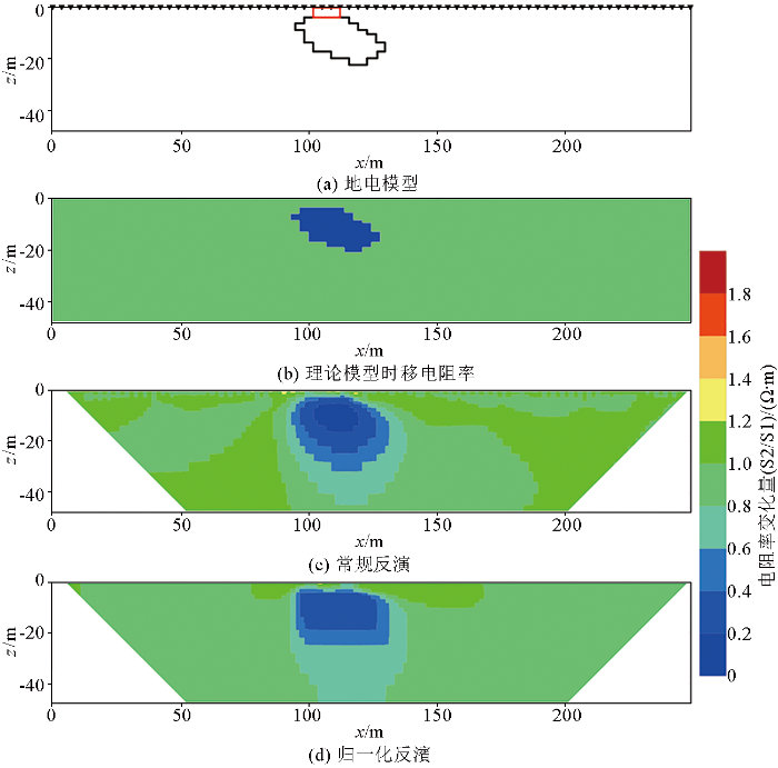
图2
理论动态模型及其时移电阻率反演结果对比
Fig.2
Comparison of different inversion methods for theoretical dynamics models and their synthetic time-lapse data
4 研究区实测方案及结果
4.1 观测方案
在北杨家桥村西侧1 km处的农田中布置了1条近SN向的高密度电阻率法测线,进行时移电阻率数据观测(图3)。测线长426 m,北端为起始端,电极距6 m,共布置电极72个。使用厘米级精度的RTK-GPS确定电极位置,确保时移测量电极位置不变,避免电极位置变化导致的数据误差。测区地形平坦,RTK-GPS定位的72个测点高程均值为27.04 m,方差0.023。由于测线布置在农田,有良好的接地条件,接地电阻都在800 Ω之内,为数据观测质量提供了保障。野外数据采集使用GD-10高密度电法仪,具体观测方案见表1。在同一极距条件下的高密度电法剖面观测中,虽然温纳装置相比偶极—偶极装置或对称四极装置的垂向分辨率更佳,有利于地下水层探测,但是其观测数据量少、探测深度小。由于初次观测方案中温纳装置的探测深度没有到达更深的含水层,因此为了研究两个含水层的电阻率结构时空分布特征,后续的观测方案中增加了偶极—偶极观测装置。
图3
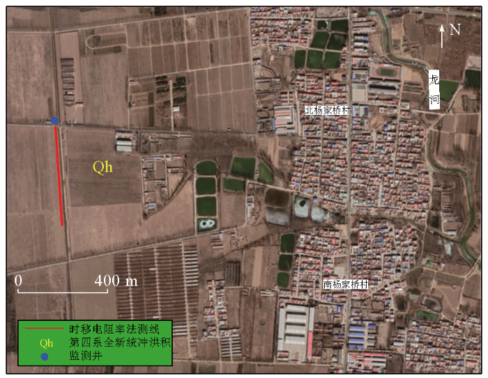
表1 时移电阻率法观测方案
Table 1
| 序号 | 观测时间 | 观测装置 | 观测方法 | 时移观 测时间 间隔/d |
|---|---|---|---|---|
| T1 | 2020-11-22 | 温纳 | 单次观测 | - |
| T2 | 2021-04-24 | 温纳、偶极—偶极 | 互换原理2次观测 | 153 |
| T3 | 2021-09-12 | 温纳、偶极—偶极 | 互换原理2次观测 | 141 |
4.2 地下含水层时空分布特征
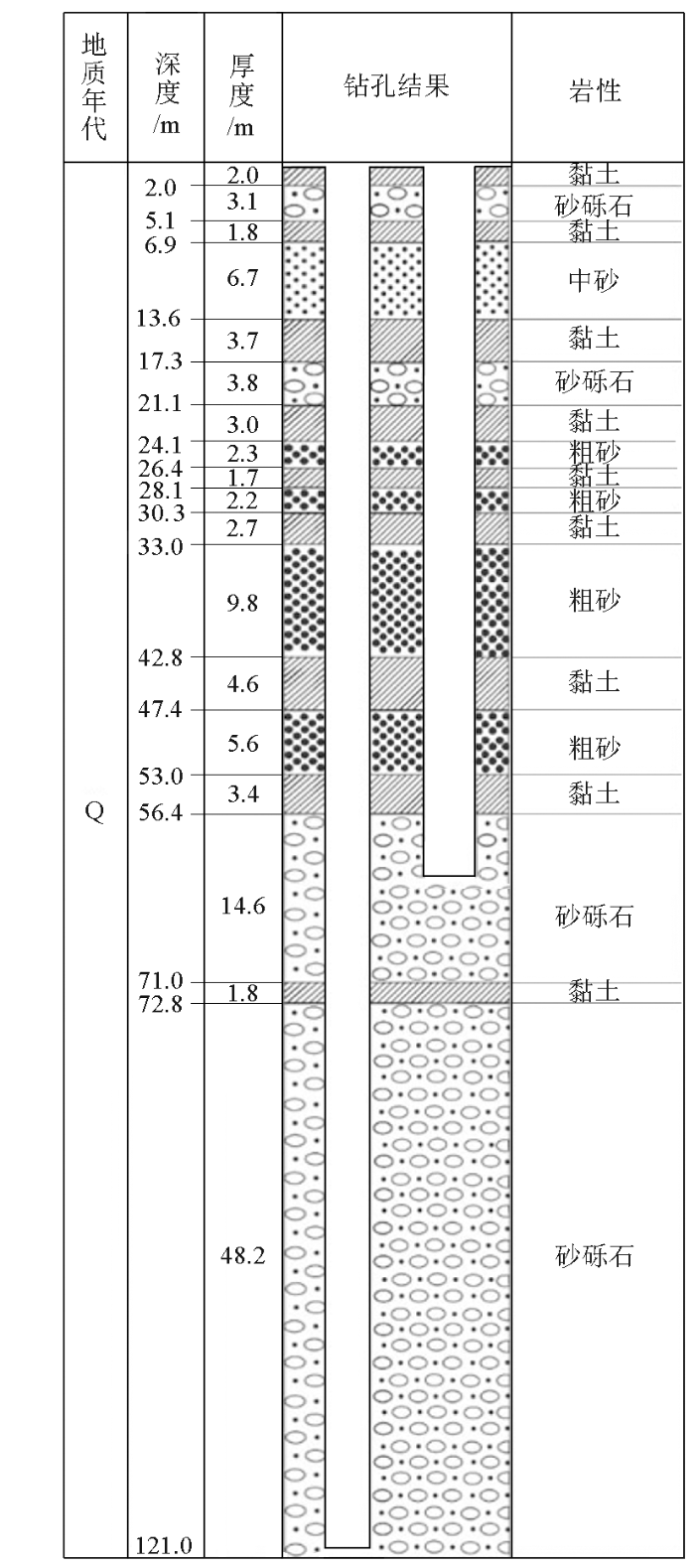
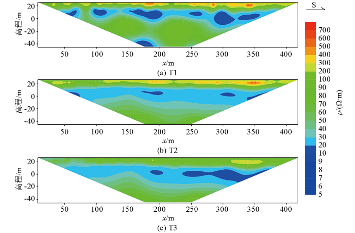
将研究区的时移温纳装置和偶极—偶极装置视电阻率数据及归一化数据进行最小二乘反演,通过常规反演结果分析地下电阻率空间结构,利用归一化数据反演结果分析地下电阻率结构变化规律。图4给出了3个时间的温纳装置数据单独反演结果,可以看出地下空间结构近似水平层状介质,高程27~20 m范围为串珠状的高阻薄覆盖层(电阻率>300 Ω∙m),高阻层下方高程15~0 m(深度12~27 m)范围内,有一个电阻率<30 Ω∙m的低阻层。根据监测井地层柱状图信息(图1)判断,高阻(红色)层为埋深0~6.9 m的包气带,由地表黏土层和砂砾石层构成,因水分含量少导致电阻率较高;低阻层(蓝色)由埋深17.3~26.4 m的粗砂层和砂砾石层构成,含水量丰富。根据反演结果可知,该低阻层为第一层含水层,水面高程约为17 m,可以判断为潜水含水层。剖面北侧的潜水面(低阻层顶界面)较南侧略高,说明该潜水含水层从北侧补给,水流方向总体上是由北向南,与研究区东侧龙河流向一致,也与研究区地下水补给方向一致(北部山区向南部平原补给)[17]。剖面其他区域(绿色)由埋深6.9~17.3 m的包气带、埋深26.4~47.4 m的粗砂与黏土互层的浅层含水层组成,相比潜水含水层,包气带和浅层含水层渗透性差、含水量较少,因此电阻率值比潜水含水层高。
图4
上述常规电阻率反演能够有效分辨出低阻潜水含水层,但无法分辨不同时间节点低阻层具体位置的差异。因此,将T1温纳装置观测数据作为背景数据,利用式(1)对T2和T3时移数据进行归一化处理(ρsh=1 Ω∙m),然后进行反演,其结果能够反映地下结构随时间的相对变化:若ρ>1 Ω∙m则空间电阻率变大,反之则空间电阻率减小。图5a中,时移数据归一化(T2/T1)反演结果反映了T1~T2期间包气带水分含量几乎不变;结合上述潜水含水层位置,该结果在潜水含水层上方出现了断续的高阻串珠状异常,高阻层下方出现低阻异常(高程范围:10~-10 m),说明潜水面水位下降,底板发生越流。图5b中,地表出现蓝色低阻薄层,表明T3比T1的降雨量和环境的湿度都有所提升,包气带中含水量增加;同样,在潜水含水层上、下分别出现了断续的高阻异常及其下方的低阻异常,相比T2/T1的结果(图5a),该高阻异常连续性更好,说明潜水面水位并没有上升,同时中部低阻纵向深度更大,表明潜水含水层进一步向承压含水层越流。
图5
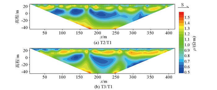
图5
温纳装置时移归一化数据反演结果
Fig.5
Inversion results of time-lapse normalized data of Wenner array
另外,在2次时移数据归一化反演结果中,高程-40 m处的高阻是由于首次观测数据质量不佳引起的,其位置与电阻率反演结果(图4a)中的不完全闭合的低阻异常一致,但是该高阻异常的范围相对较小。可见,归一化数据反演有效降低了数据噪声对反演的影响。
各时间段的温纳装置数据的单独反演和归一化数据反演结果反映了研究区包气带和潜水含水层的时空特征。在同一电极距和剖面长度下,偶极—偶极装置获得的数据量更多,探测深度更大,因此,选择在该测线进行偶极—偶极装置高密度时移视电阻率数据观测,研究承压含水层时空特征。
在T2和T3的偶极—偶极装置电阻率反演结果(图6)中,可以清晰地分辨出2个水平低阻层(<30 Ω∙m)和地表高阻薄层(>300 Ω∙m),根据监测井地质柱状图信息(图1)判断:高阻(红色)层为0~6.9 m的包气带,高程15~0 m的低阻层为潜水含水层(埋深约12~27 m),与温纳装置数据反演结果一致;高程-20~-40 m的低阻层为承压含水层,埋深47.4~71 m,由砂砾石层和粗砂层构成,与柱状图呈现的承压含水层深度范围一致;剖面其他区域(绿色)由埋深6.9~17.3 m的包气带、埋深26.4~47.4 m的粗砂与黏土互层的浅层含水层和71 m以下的深层承压水层组成,其中前两者与温纳装置数据反演结果一致,而深层承压含水层由于埋深较大,实测数据较少,导致反演结果无法分辨该含水层,因此其电阻率比上方的承压含水层高。
图6
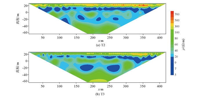
图6
偶极—偶极装置时移数据反演结果
Fig.6
Inversion results of time-lapse data of Dipole-Dipole array
将T2的偶极—偶极观测数据作为背景数据,利用式(1)对T3的时移数据进行归一化处理(ρsh=1 Ω∙m),再进行反演。时移数据归一化反演T3/T2的结果(图7)反映了包气带、潜水含水层和承压含水层水量变化规律,地表出现蓝色低值薄层,说明在T2~T3期间包气带水分含量增加; 在潜水含水层上、下分别出现了断续的高阻异常及其下方的低阻异常(高程范围0~-10 m),同样说明了潜水位下降,底板越流。该结果均与温纳装置归一化数据反演结果保持了较好的一致性(图5a和图5b)。而承压含水层位置(高程范围-20~-40 m)的电阻率值在1 Ω∙m附近,说明T2—T3期间承压含水层稳定,厚度不变,没有受到季节性降水量增大的影响。
图7
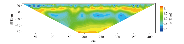
图7
偶极—偶极装置时移归一化数据(T3/T2)反演结果
Fig.7
Inversion results of time-lapse normalized(T3/T2) data of Dipole-Dipole array
5 结论与建议
1)通过对视电阻率数据进行常规反演,结合监测井岩性结果,确定了第四系地层、地下潜水含水层和承压含水层的空间分布近似为水平层状,为该区后续第四系和地下水研究工作打下基础。
2)将数据比归一化方法引入时移电阻率法数据处理,反演归一化数据后,分析了地下潜水含水层和承压含水层的季节性时空特征。本文将时移电阻率法应用于地下水动态监测,为该地区地下水的开发、管理和使用提供了重要数据支撑,也为研究地下水动态过程提供了新思路。
3)利用互换原理进行数据采集工作能够有效提升数据质量,为数据反演提供有效支撑;归一化数据反演能够有效降低数据噪声对反演的影响,缩小由数据误差引起的假构造。视电阻率数据会受到地温的影响,在时移电阻率法反演研究中应进一步考虑温度引起的数据变化。
参考文献
北京市平谷盆地地下水三维数值模拟及管理应用
[J].
Development of a 3-D numerical groundwater flow model of the Pinggu Basin and groundwater resources management
[J].
北京平谷平原区浅层地下水化学特征及成因分析
[J].
Hydrochemical characteristics of shallow groundwater and the origin in the Pinggu Plain,Beijing
[J].
北京平原区地下水位预警初步研究
[J].
A preliminary study of groundwater level pre-warning in Beijing Plain
[J].
北京平原地下水可持续开采方案分析
[J].
Analysis of sustainable groundwater resources development scenarios in the Beijing Plain
[J].
Hydrological response of weathered clay-shale slopes:water infiltration monitoring with time-lapse electrical resistivity tomography
[J].DOI:10.1002/hyp.v26.14 URL [本文引用: 1]
Landslide monitoring in southwestern China via time-lapse electrical resistivity tomography
[J].DOI:10.1007/s11770-016-0543-3 URL [本文引用: 1]
4D electrical resistivity tomography monitoring of soil moisture dynamics in an operational railway embankment
[J].
DOI:10.3997/1873-0604.2013002
URL
[本文引用: 1]

The internal moisture dynamics of an aged (> 100 years old) railway earthwork embankment, which is still in use, are investigated using 2D and 3D resistivity monitoring. A methodology was employed that included automated 3D ERT data capture and telemetric transfer with on‐site power generation, the correction of resistivity models for seasonal temperature changes and the translation of subsurface resistivity distributions into moisture content based on petrophysical relationships developed for the embankment material. Visualization of the data as 2D sections, 3D tomo‐grams and time series plots for different zones of the embankment enabled the development of seasonal wetting fronts within the embankment to be monitored at a high‐spatial resolution and the respective distributions of moisture in the flanks, crest and toes of the embankment to be assessed. Although the embankment considered here is at no immediate risk of failure, the approach developed for this study is equally applicable to other more high‐risk earthworks and natural slopes.
A clustering approach applied to time-lapse ERT interpretation—Case study of Lascaux cave
[J].DOI:10.1016/j.jappgeo.2017.07.006 URL [本文引用: 1]
A case study of resistivity and self-potential signatures of hydrothermal instabilities,Inferno Crater Lake,Waimangu,New Zealand
[J].DOI:10.1029/2009GL037573 URL [本文引用: 1]
Evaluating four-dimensional time-lapse electrical resistivity tomography for monitoring DNAPL source zone remediation
[J].
Improved time-lapse electrical resistivity tomography monitoring of dense non-aqueous phase liquids with surface-to-horizontal borehole arrays
[J].DOI:10.1016/j.jappgeo.2014.10.022 URL [本文引用: 1]
Seasonal groundwater recharge characterization using time-lapse electrical resistivity tomography in the Thepkasattri watershed on Phuket Island,Thailand
[J].
Using time-lapse resistivity imaging methods to quantitatively evaluate the potential of groundwater reservoirs
[J].
DOI:10.3390/w14030420
URL
[本文引用: 1]
In this study, we attempt to establish an alternative method for estimating the groundwater levels and the specific yields of an unconfined aquifer for the evaluation of potential groundwater reservoirs. We first converted the inverted resistivity into the normalized water content. Then, we inverted the parameters of the Brooks-Corey model from the vertical profiles of the water content by assuming that the suction head was in proportion to the elevation regarding a predefined base level. Lastly, we estimated the groundwater level, the theoretical specific yield, and the specific yield capacity from the Brooks-Corey parameters at every survey site in the study area. The contour maps of the time-lapse groundwater levels show that the groundwater flows downstream, with a higher hydraulic gradient near the river channel than in the area away from the main channel. We conclude that the estimated maximum specific yield capacities are consistent with that derived from the pumping tests in the nearby observation well. Additionally, the specific yield capacities are only three quarters to two thirds of the theoretical specific yields derived from the difference between the residual and saturated water contents in the Brooks-Corey model. We conclude that the distribution pattern of the specific yields had been subjected to the distribution of natural river sediments in the Minzu Basin, since the modern channel was artificially modified. Although we had to make some simple assumptions for the estimations, the results show that the surface resistivity surveys provide reasonable estimations of the hydraulic parameters for a preliminary assessment in an area with few available wells.
Groundwater flow monitoring using time-lapse electrical resistivity and self potential data
[J].DOI:10.1016/j.jappgeo.2021.104411 URL [本文引用: 1]
Characterization of groundwater and surface water mixing in a semiconfined karst aquifer using time-lapse electrical resistivity tomography
[J].DOI:10.1002/wrcr.v50.3 URL [本文引用: 1]
Spatial monitoring of groundwater drawdown and rebound associated with quarry dewatering using automated time-lapse electrical resistivity tomography and distribution guided clustering
[J].
环境同位素在北京平谷盆地山前侧向补给研究中的应用
[J].
Application of environmental isotopes in the study of lateral recharge in front of Pinggu basin Beijing
[J].
三河—平谷8级大震区地壳上地幔电性结构特征研究
[J].
Electrical structures of the crust and upper mantle in Sanhe-Pinggu M8 earthquake area,China
[J].
Electrical resistivity tomography of vadose water movement
[J].DOI:10.1029/91WR03087 URL [本文引用: 1]
Application of time-lapse ERT imaging to watershed characterization
[J].
DOI:10.1190/1.2907156
URL
[本文引用: 1]
Time-lapse electrical resistivity tomography (ERT) has many practical applications to the study of subsurface properties and processes. When inverting time-lapse ERT data, it is useful to proceed beyond straightforward inversion of data differences and take advantage of the time-lapse nature of the data. We assess various approaches for inverting and interpreting time-lapse ERT data and determine that two approaches work well. The first approach is model subtraction after separate inversion of the data from two time periods, and the second approach is to use the inverted model from a base data set as the reference model or prior information for subsequent time periods. We prefer this second approach. Data inversion methodology should be consideredwhen designing data acquisition; i.e., to utilize the second approach, it is important to collect one or more data sets for which the bulk of the subsurface is in a background or relatively unperturbed state. A third and commonly used approach to time-lapse inversion, inverting the difference between two data sets, localizes the regions of the model in which change has occurred; however, varying noise levels between the two data sets can be problematic. To further assess the various time-lapse inversion approaches, we acquired field data from a catchment within the Dry Creek Experimental Watershed near Boise, Idaho, U.S.A. We combined the complimentary information from individual static ERT inversions, time-lapse ERT images, and available hydrologic data in a robust interpretation scheme to aid in quantifying seasonal variations in subsurface moisture content.
Electrical resistance tomography
[J].DOI:10.1190/1.1729225 URL [本文引用: 1]
Difference inversion of ERT data:a fast inversion method for 3-D in situ monitoring
[J].
DOI:10.4133/JEEG6.2.83
URL
[本文引用: 1]
A three-dimensional (3-D) Occam’s inversion algorithm for electrical resistivity tomography is modified to allow for inversion on the differences between the background and subsequent data sets. The algorithm is optimized for in situ monitoring applications. The resistivity obtained by the inversion of background data serves as the a priori model in the difference inversion. There are several advantages to this method. First, convergence is fast since the inverse routine needs only to find small perturbations about a good initial guess. Second, systematic errors such as those due to errors in field configuration and discretization errors in the forward modeling algorithm tend to cancel. The result is that we can fit the difference data far more closely than the individual potentials. Better data fits often equate to better resolution with fewer inversion artifacts. The difference inversion technique was applied to monitoring in-situ steam remediation in Portsmouth, Ohio and monitoring of flow in fluid fractures at the Box Canyon site near the Idaho National Engineering Laboratory. Small changes of conductivity were better resolved using the difference inversion method. Difference inversion produced high-quality images with fewer artifacts, and only took 25% to 50% run time of standard Occam’s inversion in the Box Canyon case.
A saline trace test monitored via time-lapse surface electrical resistivity tomography
[J].DOI:10.1016/j.jappgeo.2005.10.007 URL [本文引用: 1]
时移电阻率法归一化数据反演分辨电阻率结构微小变化
[J].
The normalized data inversion of time-lapse resistivity method for resolving small resistivity changes
[J].
4-D inversion of DC resistivity monitoring data acquired over a dynamically changing earth model
[J].DOI:10.1016/j.jappgeo.2009.03.002 URL [本文引用: 1]
Simultaneous time-lapse electrical resistivity inversion
[J].DOI:10.1016/j.jappgeo.2011.06.035 URL [本文引用: 1]
A comparison of the gauss-newton and quasi-newton methods in resistivity imaging inversion
[J].DOI:10.1016/S0926-9851(01)00106-9 URL [本文引用: 1]
The effects of noise on Occam’s inversion of resistivity tomography data
[J].
DOI:10.1190/1.1443980
URL
[本文引用: 1]
An Occam’s inversion algorithm for crosshole resistivity data that uses a finite‐element method forward solution is discussed. For the inverse algorithm, the earth is discretized into a series of parameter blocks, each containing one or more elements. The Occam’s inversion finds the smoothest 2-D model for which the Chi‐squared statistic equals an a priori value. Synthetic model data are used to show the effects of noise and noise estimates on the resulting 2-D resistivity images. Resolution of the images decreases with increasing noise. The reconstructions are underdetermined so that at low noise levels the images converge to an asymptotic image, not the true geoelectrical section. If the estimated standard deviation is too low, the algorithm cannot achieve an adequate data fit, the resulting image becomes rough, and irregular artifacts start to appear. When the estimated standard deviation is larger than the correct value, the resolution decreases substantially (the image is too smooth). The same effects are demonstrated for field data from a site near Livermore, California. However, when the correct noise values are known, the Occam’s results are independent of the discretization used. A case history of monitoring at an enhanced oil recovery site is used to illustrate problems in comparing successive images over time from a site where the noise level changes. In this case, changes in image resolution can be misinterpreted as actual geoelectrical changes. One solution to this problem is to perform smoothest, but non‐Occam’s, inversion on later data sets using parameters found from the background data set.
