|
|
|
| Method for accurately calculating magnetic anomaly component using ΔT based on L-BFGS inversion algorithm |
Hui-Xiang ZHEN, Yu-Shan YANG( ), Yuan-Yuan LI, Tian-You LIU ), Yuan-Yuan LI, Tian-You LIU |
| Institute of Geophysics and Geomatics, China University of Geosciences(Wuhan), Wuhan 430074, China |
|
|
|
|
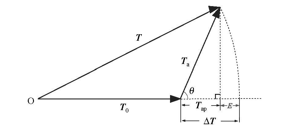
Abstract In the magnetic exploration theory, total-field anomaly ΔT is regarded as the component Tap of the magnetic anomaly vector Ta on the main field (T0) direction and thus constitutes the theoretical basis. However, there is an error in this approximation. Theoretical calculations and experiments have proved that this approximation error will increase rapidly as the Ta increases. When the magnetic anomaly Ta is much smaller than T0, the influence of the error is small and negligible. In the case of a strong magnetic anomaly, the error is large, and the processing interpretation accuracy of the ΔT anomaly is greatly affected. For high-precision magnetic exploration, ΔT must be converted to a magnetic anomaly component Tap for processing and interpretation. In this paper, the method of accurately calculating the magnetic anomaly component using Tap based on the Limited-memory Broyden-Fletcher-Goldfarb-Shanno (L-BFGS) algorithm is proposed. Firstly, the authors derived the forward formula for ΔT from Tap, and then constructed the objective function of Tap inversion by the difference function between ΔT and Tap. L-BFGS algorithm was used to solve the Tap from ΔT. Model experiments show that the Tap calculated by this method is very close to the real value, which can reduce the error by two orders of magnitude. This method also yields good results in the presence of noise and background fields. The method was applied to the processing of ΔT magnetic survey data of the Yangshan iron mine in Fujian Province, and the results of processing and interpretation which are more consistent with the actual results were obtained.
|
|
Received: 24 October 2018
Published: 31 May 2019
|
|
|
|
Corresponding Authors:
Yu-Shan YANG
E-mail: samyys@126.com
|
|
|
|

|
Schematic diagram of total field anomaly ΔT and other related physical quantities
|
|
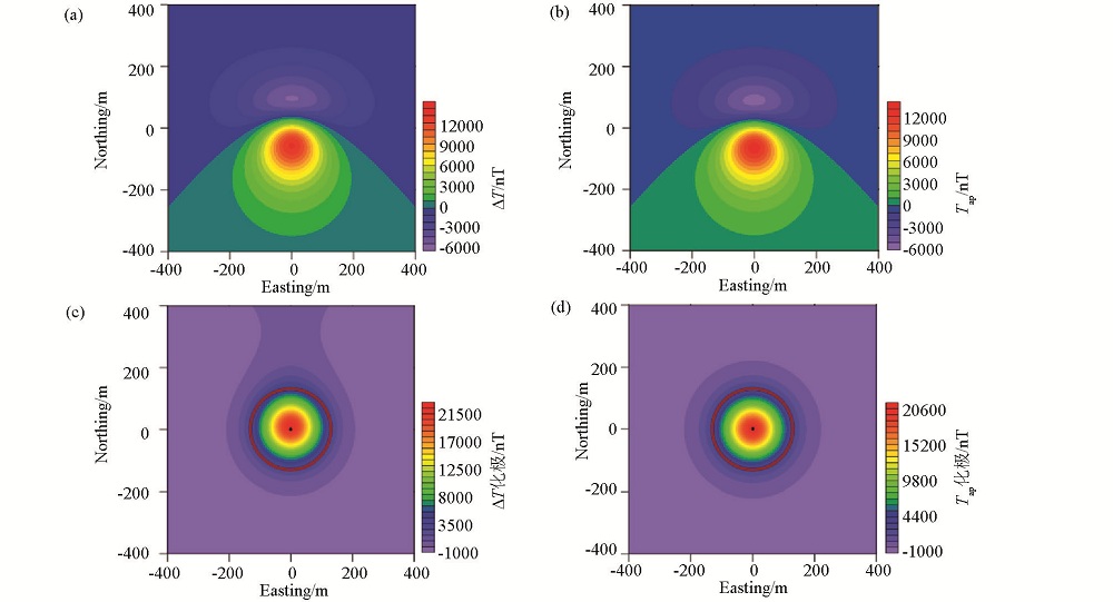
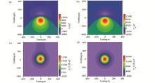
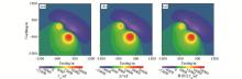
Reduction to the pole (RTP) results comparison of ΔT and Tap under strong magnetic anomalies
a—ΔT of the sphere model; b—Tap of the sphere model; c—RTP of the sphere model ΔT; d—RTP of the sphere model Tap;the red circle in the figure represents the projection of the sphere model and the black dot represents the midpoint of the sphere model
|

| 模型 | 中心X坐标
/m | 中心Y坐标
/m | 半径
/m | 中心埋深
/m | 磁化强度J
/(A·m-1) | | 单球体模型 | 50 | 50 | 250 | 300 | 120 | | 组合模型A | -300 | 300 | 250 | 350 | 120 | | 组合模型B | 300 | -300 | 400 | 500 | 120 |
|
Model geometric parameters of and magnetization
|
|
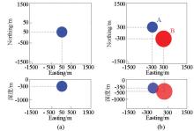
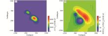
Model horizontal and profile projection
a—single sphere model; b—combined sphere model
|
|
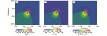
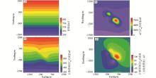
Comparison of Tap, ΔT and calculated Tap
a—the projection component Tap of the magnetic anomaly in the direction of the normal geomagnetic field; b—the total field anomaly ΔT; c—the magnetic anomaly component Tap obtained by the inversion
|

|
Single sphere model inversion error
a—difference between ΔT and Tap (ie, initial deviation); b—error between the inverted Tap and the theoretical Tap
|
|
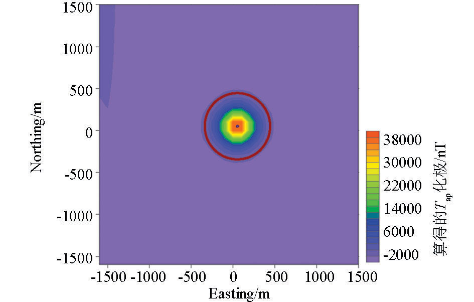
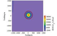
The result of the inversion of the magnetic anomaly component Tap
The red circle in the figure represents the projection of the sphere model, and the black dot represents the midpoint of the sphere model
|
|
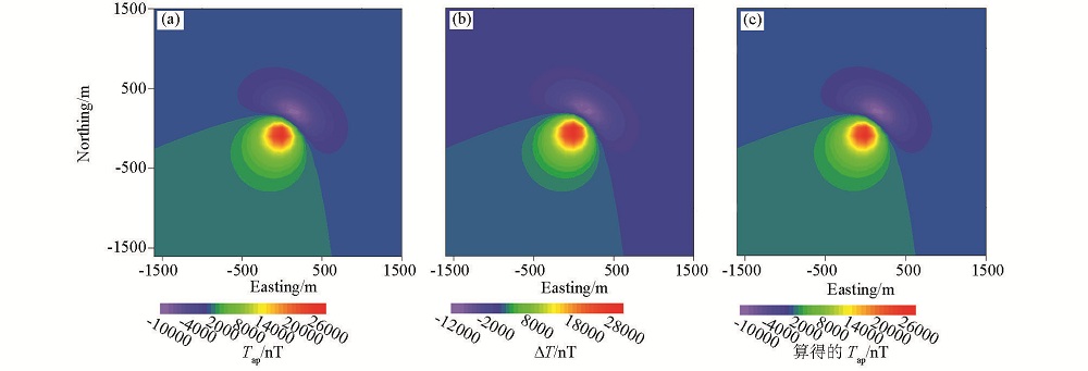
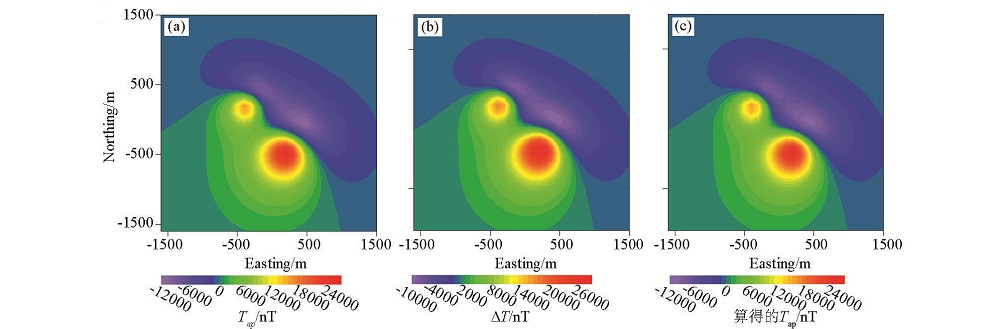
Comparison of Tap, ΔT and calculated Tap
a—the projection component Tap of the magnetic anomaly in the direction of the earth’s magnetic field; b—the total field anomaly ΔT; c—the magnetic anomaly component Tap obtained by the inversion
|
|
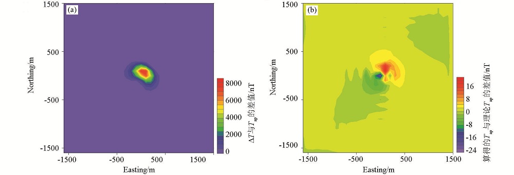
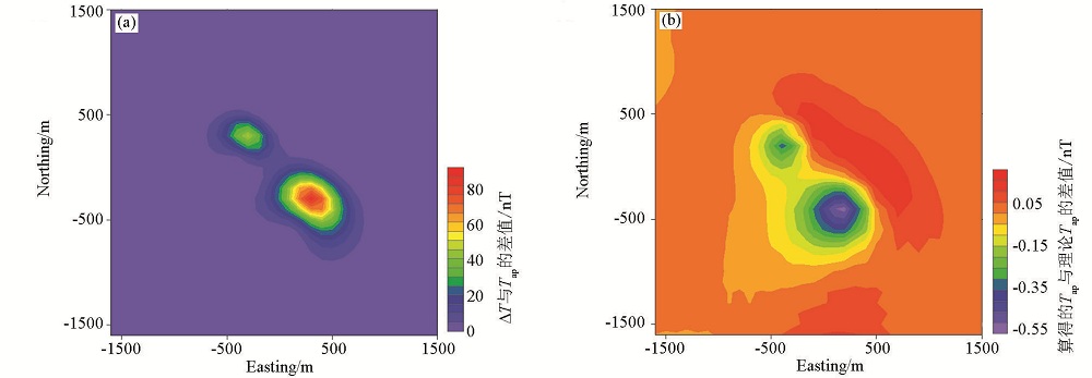
Inversion error of combined sphere model
a—difference between ΔT and Tap (ie, initial deviation); b—error between the inverted Tap and the theoretical Tap
|

|
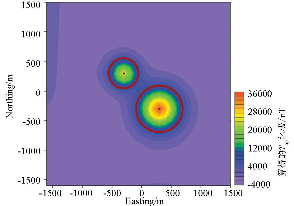
The RTP result of the magnetic anomaly component Tap obtained by inversion
The red circle in the figure represents the projection of the sphere model, and the black dot represents the midpoint of the sphere model
|

|
error of Tap obtained by inversion of combined sphere model under weak magnetic anomaly
a—difference between ΔT and Tap (ie, initial deviation); b—error between the inverted Tap and the theoretical Tap
|

|
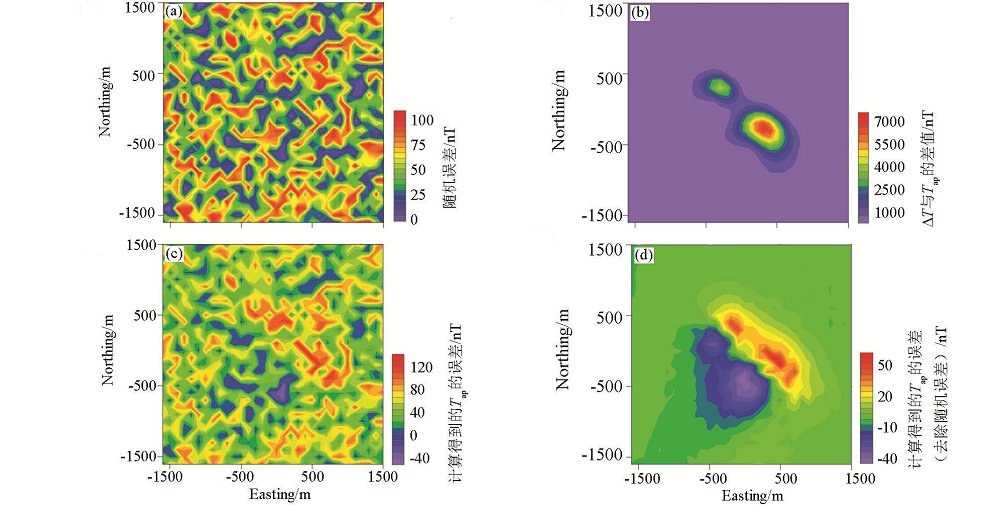
Model experiment for superimposed noise
a—0~100 nT random noise; b—approximation error of ΔT superimposed with random noise; c—error of Tap obtained by ΔT inversion of superimposed noise; d—Tap error result obtained by inversion (after noise elimination)
|
|
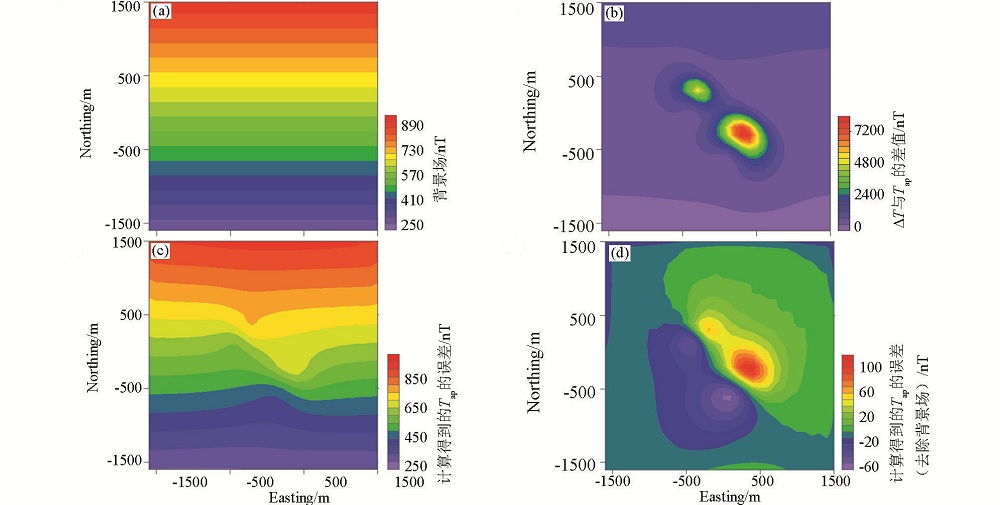
The model experiment of the superimposed background field
a—the background field; b—approximation error of ΔT (overlay background field); c—error of Tap obtained by ΔT inversion of superimposed background field; d—Tap error result obtained by inversion (after eliminating the background field)
|
|
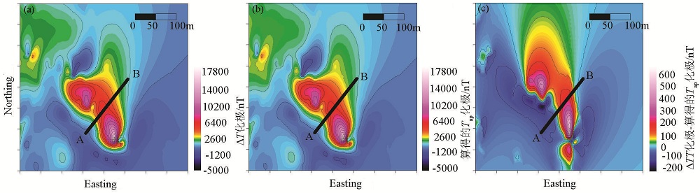
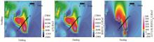
Comparison of ΔT reduction to the pole result of measured data and Tap RTP result obtained by inversion
a—ΔT RTP result of measured data; b—Tap RTP result obtained by inversion; c—difference between two polarization results
|
|
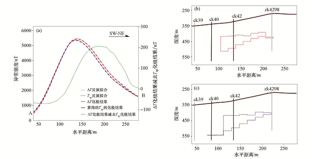
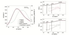
Profile inversion comparison of ΔT and calculated Tap
a—ΔT reduction to the pole curve, Tapreduction to the pole curve and their inversion fitting results along the section AB; b—inversion result of the observed ΔT data; c—inversion result of the calculated Tap data; See ore through dring bore ck40, ck42, no mine ore is found in borehole ck39, zk4298
|
| [1] |
Parasnis D S . Principles of Applied Geop[M]. Berlin: Springer Netherlands, 1979.
|
| [2] |
管志宁 . 我国磁法勘探的研究与进展[J]. 地球物理学报, 1997,40(1):299-307.
|
| [2] |
Guan Z N . Research and development of magnetic law exploration in China[J]. Chinese Journal of Geophysics, 1997,40(1):299-307.
|
| [3] |
Blakely R J. Potential theory in gravity and magnetic applications[M]. Cambridge: Cambridge University Press, 1995.
|
| [4] |
管志宁 . 地磁场与磁力勘探[M]. 北京: 地质出版社, 2005.
|
| [4] |
Guan Z N. Geomagnetic field and magnetic exploration [M]. Beijing: Geological Press, 2005.
|
| [5] |
刘天佑 . 磁法勘探[M]. 北京: 地质出版社, 2013.
|
| [5] |
Liu T Y. Magnetic exploration[M]. Beijing: Geological Press, 2013.
|
| [6] |
Hinze P W J, Von Frese R R B, Saad A H . Gravity and magnetic exploration: principles, practices, and applications[M]. Cambridge: Cambridge University Press, 2013.
|
| [7] |
塔费耶夫 . 金属矿床的地球物理勘探文选[M]. 北京: 地质出版社. 1954.
|
| [7] |
Tafeev. A geophysical exploration of metal deposits[M]. Beijing: Geological Publishing House. 1954.
|
| [8] |
袁晓雨, 姚长利, 郑元满 , 等. 强磁性体ΔT异常计算的误差分析研究[J]. 地球物理学报, 2015,58(12):4756-4765.
|
| [8] |
Yuan X Y, Yao C L, Zheng Y M , et al. Error analysis of ΔT anomaly calculation of ferromagnetic body[J]. Chinese Journal of Geophysics, 2015,58(12):4756-4765.
|
| [9] |
袁晓雨 . 强磁异常ΔT的计算误差及高精度处理转换分析研究[D]. 中国地质大学 (北京), 2016.
|
| [9] |
Yuan X Y . Research on calculation error and high-precision processing conversion analysis of strong magnetic anomaly ΔT [D]. China University of Geosciences ( Beijing), 2016.
|
| [10] |
Baranov W A . New method for interpretation of aeromagnetic maps: pseudo-gravimetric anomalies[J]. Geophysics, 1957,22(2):359-383.

|
| [11] |
Bhattacharyya B K . Two-dimensional harmonic analysis as a tool for magnetic interpretation[J]. Geophysics, 1965,30(5):829-857.
|
| [12] |
袁亚湘, 孙文瑜 . 最优化理论与方法[M]. 北京: 科学出版社, 1997.
|
| [12] |
Yuan Y X, Sun W Y. Optimization theory and method[M]. Beijing: Science Press, 1997.
|
| [13] |
Sun W, Yuan Y X . Optimization theory and methods[M]. New York: Springer US, 2006: 175-200.
|
| [14] |
姚姚 . 地球物理反演[M]. 北京: 中国地质大学出版社, 2002.
|
| [14] |
Yao Y. Geophysical inversion[M]. Beijing: China University of Geosciences Press, 2002.
|
| [15] |
王家映 . 地球物理反演理论[M]. 北京: 高等教育出版社, 2002.
|
| [15] |
Wang J Y , Geophysical inversion theory[M]. Beijing: Higher Education Press, 2002.
|
| [16] |
Avdeeva A, Avdeev D . A limited-memory quasi-Newton inversion for 1D magnetotellurics[J]. Geophysics, 2006,71(5):G191-G196.
|
| [17] |
张生强, 刘春成, 韩立国, 等 . 基于 L-BFGS 算法和同时激发震源的频率多尺度全波形反演[J]. 吉林大学学报: 地球科学版, 2013,43(3):1004.
|
| [17] |
Zhang S Q, Liu C C, Han L G , et al. Frequency multi-scale full waveform inversion based on L-BFGS algorithm and simultaneous excitation source[J]. Journal of Jilin University: Earth Science Edition, 2013,43(3):1004.
|
| [18] |
Broyden C G . The convergence of a class of double-rank minimization algorithms[J]. Journal of the Institute of Mathematics and Its Applications, 1970(6):76-90.
|
| [19] |
Fletcher R . A new approach to variable metric algorithms[J]. Computer Journal, 1970,13(3):317-322.
|
| [20] |
Goldfarb D . A family of variable metric updates derived by variational means[J]. Mathematics of Computation, 1970,24(109):23-26.
|
| [21] |
Shanno D F . Conditioning of quasi-Newton methods for function minimization[J]. Mathematics of Computation, 1970,24(111):647-656.
|
| [22] |
Zheng Y K, Wang Y, Chang X . Wave-equation traveltime inversion: comparison of three numerical optimization methods[J]. Computers & Geosciences, 2013,60(10):88-97.
|
| [23] |
Fabien-Ouellet G, Gloaguen E, Giroux B . A stochastic L-BFGS approach for full-waveform inversion[J]. Seg Technical Program Expanded, 2017: 1622-1627.
|
| [24] |
Dong C, Liu J N . On the limited memory BFGS method for large scale optimization[J]. Mathematicial Programming, 1989,45(1-3):503-528.
|
| [25] |
Nocedal J . Upgrading quasi-newton matrices with limited storage[J]. Mathematics of Computation, 1980,35(151):773-782.
|
| [26] |
Nocedal J, Wright S J . Numerical optimization[M]. New York: Springer, 2006.
|
| [27] |
Pan W, Innanen K A, Liao W . Accelerating hessian-free gauss-newton full-waveform inversion via L-BFGS preconditioned conjugate-gradient algorithm[J]. Geophysics, 2017,82(2):R49-R64.
|
|
|
|