

0 引言
地球物理联合反演是利用多种方式采集所取得的数据来实现多种物性参数反演的方法[1]。在综合地球物理勘探中,联合反演是一种重要的定量解释手段,近些年的大量研究结果表明,联合反演方法能够较好地压制干扰信息(如背景噪声),减小地球物理反演问题中的多解性,获取更为可靠、精准的反演结果,可进一步提高反演解释的精度[2⇓-4]。国外学者对于海洋可控源电磁法(marine controllable source electromagnetic method,MCSEM)和地震资料的联合反演有一定的研究:Hu等[5]成功实现了基于交叉梯度的MCSEM资源和地震走时资料的交互式联合反演(alternating joint inversion),成像精度有显著提升;Brown等[6]实现了地震全波形资料约束MCSEM资料的二维Occam反演,利用澳大利亚Pluto气田数据反演结果验证了该方法的有效性;Da Silva等[7]实现了使用地震全波形资料约束的MCSEM三维反演,并取得了较好的成果;Mac-Gregor等[8]应用Archie公式来估算西非某海域海底底层的电阻率和地震波速度之间的经验关系。然而,这些研究主要还是基于岩石物理关系的同步联合反演,这种方法过于依赖电阻率和地震波波速之间的岩石物理关系[9]。
本文在前人提出的交叉梯度的基础上,建立了基于交叉梯度函数约束的MCSEM和地震全波形反演的目标函数,详细推导了梯度表达式,实现地下电阻率和地震波速度这两种物性参数之间相互约束的联合反演算法,并通过理论模型的测试,探讨了联合反演算法的可行性及适用性。
1 地震全波形和海洋可控源电磁二维正反演方法
1.1 地震全波形二维正反演方法
1.2 海洋可控源电磁二维正反演方法
对于MCSEM中二次场的计算,本文使用基于四边形网格剖分的有限单元法[20]:在二维空气—海水—海底岩石的层状模型中,设走向方向为y,水平电偶源位于海底上方的海水中,产生如下关于
式中:
利用加权余量法对有限元方程进行了推导。参照Mitsuhata[20],本文同样使用伽辽金法,将格林公式加入到式(1)中,对所有网格单元进行叠加,并考虑到如下边界条件:在内边界上,电场和磁场的切向分量(
式中:Ne表示网格单元的总数。
数据空间Occam反演理论是由Siropunvarapor W与Egbert G[21]在传统Occam反演方法的基础上提出来的,该方法改进了模型空间Occam反演方法,是通过数学方法将模型迭代更新公式的计算和储存从模型空间转换到数据空间,这种数学转换不仅降低了计算量和存储空间,同时也提高了计算效率。
数据空间Occam反演流程如下:首先,输入观测参数以及初始模型(ρ0),计算雅可比矩阵(Jk),这里使用自动搜索的方式获取了拉格朗日算子(λ),并计算当前模型响应的数据拟合差(RMS),同时选择RMS最小时所对应的λ值;然后,根据当前的λ值更新电阻率模型。为提高计算效率,选择当反演迭代次数满足所规定的最大值时终止迭代进程,并输出反演模型。
2 基于交叉梯度耦合的二维联合反演方法
2.1 二维交叉梯度函数
交叉梯度函数是由Meju与Gallardo等[22]首次提出的:
式中:mr、mv表示2种不同的参与联合反演的物性参数,他们在空间上的分布是已知的,文中这2种物性参数分别为取对数的电阻率和取对数的速度;Ñ表示对模型参数取梯度。
对于二维模型,设地质体走向方向为沿y轴正方向,模型在y方向上的偏导数为0,那么t在x及z方向上的分量均为0,只有y方向上有值,即
使用中心差分格式将方程(5)进行如图1所示的离散化处理,mr与mv共用一套相同的网格,其中的网格可以是等间距剖分也可以是不等间距剖分。
图1
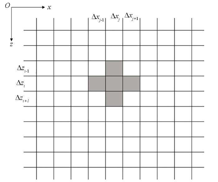
用差商替代微商,得到交叉梯度函数的数值表达式:
式中:i、j分别表示z方向和x方向的网格数目。
为验证上述交叉梯度算法的正确性,建立了如图2所示的2种模型Model 1和Model 2。其中,Model 1的模型参数从中心开始,以放射状向周围递增,Model 2的模型参数呈水平状分布,由浅至深逐增;2组模型具有相同的网格剖分。
图2
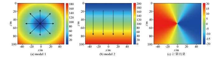
对这2个模型进行交叉梯度计算,结果如图2c所示:在中心位置的垂直方向上,即2组模型参数的梯度方向相互平行时,其交叉梯度值为零;当2种模型参数的梯度方向存在一定夹角时,其交叉梯度值不为零,且随着角度的增大而增大;当在深度为50 m处即梯度方向相互垂直时,交叉梯度值达到最大。
2.2 联合反演网格
全波形反演使用等间距网格进行剖分,边界条件采用的是PML吸收边界条件。海洋可控源电磁法的单方法反演,其异常区域内的网格是等间距的,垂直向下以及水平两端方向上的网格是不等间距的,且离异常体的距离越远间距越大,边界条件采用的是Dirichlet外边界条件。2种方法在进行交叉梯度计算时选取公共网格,对于其他部分,令交叉梯度的权重因子为0。
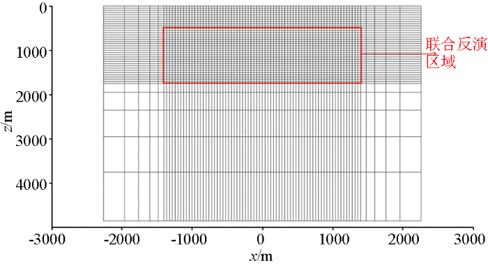
在进行MCSEM与地震全波形二维联合反演时,采用如图3所示的反演网格:红色线框内为计算交叉梯度的网格,就是地震全波形所剖分的网格与MCSEM的等间距网格的重合部分,即联合反演区域,剩余部分的网格为MCSEM反演扩充区域。
图3
2.3 联合反演理论
基于海洋可控源电磁法与地震全波形的联合反演,并结合两者反演的目标函数,构建如下基于交叉梯度约束的联合反演目标函数:
其中:
式中:
由此可见,通过交叉梯度函数耦合两种物性,在单方法反演过程中受到另外一种方法反演结果的影响,增强了两种方法之间反演结果在结构上的一致性。
其中:
求取每个网格单元的ti,j并将对应位置相加,式(11)、(12)可简化为
式中:Wr,cross与Wv,cross为交叉梯度的系数矩阵,Wr,cross与速度模型mv的参数信息相关,Wv,cross与电阻率模型mr的参数信息相关。在式(14)的基础上,将交叉梯度函数对模型向量求偏导,得到:
对目标函数式(7)求取关于
令
对目标函数式(7)求取关于
其关于
进而可得到速度模型的最终迭代公式:
在式(17)、(20)的基础上完成基于交叉梯度约束的MCSEM与地震全波形的二维联合反演研究。
2.4 联合反演流程
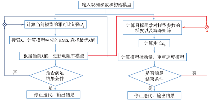
联合反演流程如图4所示。首先,输入观测参数和初始模型:对参数进行初始化,MCSEM和地震全波形分别输入电阻率和速度的海底空间模型,然后进行一次地震频率域全波形反演,得到速度模型,利用该速度模型去计算交叉梯度,以此来约束MCSEM的反演;在完成一次模型的更新后,将更新了的电阻率模型加至地震全波形反演中,并计算交叉梯度达到更新速度模型的效果;两种反演方法交替迭代进行,相互约束,直至反演迭代满足本文中所设定的终止要求(即最大迭代次数)。
图4
3 算例分析
3.1 单一板状体模型算例
建立如图5所示的高阻低速板状体理论模型,模拟海底地层中的油气储层构造。
图5
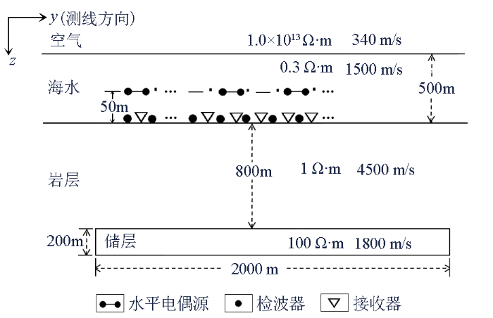
设模型海水层深500 m,电阻率为0.3 Ω·m,速度为1 500 m/s;在海底之下800 m处有一个厚200 m、横向宽度2 000 m、电阻率100 Ω·m、速度1 800 m/s的储层;背景电阻率为1 Ω·m,速度为4 500 m/s。接收器布置在海底,沿测线方向每隔100 m放置一个,共计41个(-2~2 km);水平电偶源放置在距离海底50 m的高度上,长度为1 m,电流为1 A,沿测线方向设置21个发射源,间隔200 m(-2~2 km),发射频率分别为0.25、0.5、1.5 Hz。地震全波形使用海底放炮、海底接收的观测方式,检波器同样设置在海底沿y轴-2~2 km范围内,道间距100 m,共计41个;炮点沿海底面测线方向(-2~2 km) 设置41个,炮间距100 m。
理论模型正演数据(Ey的实部和虚部)加入2%的噪声作为观测数据进行反演;取1、2、3、5、6、8和10 Hz共7个频率进行反演。地震全波形使用51×81的均匀网格进行剖分,大小为100 m×100 m;MCSEM使用的网格大小为49×69,为不等间距网格,与地震全波形网格剖分的异常区域是相同的。MCSEM和地震全波形的反演初始模型均为空气—海水—岩层模型,反演设置在25次迭代后停止。MCSEM和地震全波形的反演结果见图6。
图6
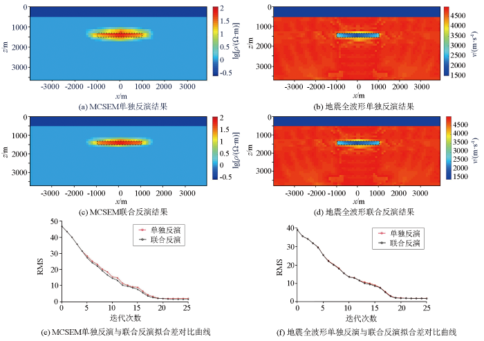
图6
单一板状体模型反演结果及拟合差迭代曲线
Fig.6
The profile of the inversion as well as the iterative curve of the RMS misfit of the single tabular body model
图6e、f给出了MCSEM、地震全波形反演的数据拟合差收敛曲线。反演过程中,两种方法的RMS值均稳定下降,在后期趋于稳定,其中MCSEM单独反演的RMS值降到1.88,联合反演的RMS值降到约1.42;地震全波形单独反演与联合反演的RMS曲线基本重合,迭代22次后RMS值稳定在1.35。
3.2 复杂板状体模型算例
建立如图7所示的复杂板状体理论模型,模拟海底地层中存在上覆异常体的油气储层。
图7
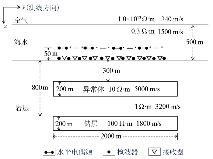
海水层深500 m,电阻率为0.3 Ω·m,速度为1 500 m/s;海底300 m处有一个厚200 m、横向宽度2 000 m、电阻率10 Ω·m、速度5 000 m/s的低阻高速板状体,在其下方500 m处有一个厚200 m、横向宽度2 000 m、电阻率100 Ω·m、速度1 800 m/s的高阻低速板状体;背景电阻率为1 Ω·m,速度为3 200 m/s。地震与MCSEM的观测系统、反演网格和迭代次数的设置与3.1节相同。
MCSEM和地震的反演结果见图8。MCSEM单独反演结果中的异常体整体形态与理论模型偏差较大,收敛性很差,上层低阻板状体没有显示出来,下层高阻板状体反演后的位置在1 200 m处(图8a),这主要是由于上层低阻板状体对下层高阻板状体的影响使得高阻板状体的位置与原始模型有较大的偏差,电阻率值在15~60 Ω·m,周围存在较大的冗余构造。联合反演的结果明显改善了异常体的位置信息以及模型的形态,虽然对于上层的低阻板状体反演效果还是较差,仅仅是电阻率值稍有改善,但是对于下层高阻板状体的位置,形状都基本恢复了(图8c),其电阻率异常值为50~80 Ω·m,对真值的恢复能力有了明显的提高,并且明显压制了周围的虚假异常。而地震的单方法反演对异常体的速度和边界的恢复效果较好,只是异常体周围存在少许的假异常(图8b),联合反演速度结果相比于单方法没有明显的提高(图8d)。
图8
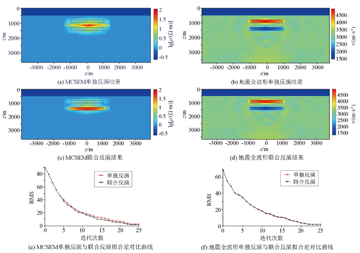
图8
复杂板状体模型反演结果及拟合差迭代曲线
Fig.8
The profile of the inversion as well as the iterative curve of the RMS misfit of the complex tabular body model
图8e、f给出了MCSEM与地震全波形反演的数据拟合差收敛曲线,可以发现在反演过程中,MCSEM的 RMS值前期下降速度较快,在后期趋于稳定,其单独反演的RMS值降到2.85,联合反演的RMS值下降到1.78;地震全波形单独反演与联合反演的RMS曲线基本重合,迭代24次后RMS值稳定在1.63。
3.3 凹槽体模型算例
建立如图9所示的低阻低速凹槽体理论模型,模拟海底地层中的背斜构造。
图9
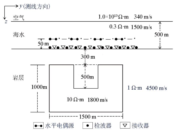
海水层深为500 m,电阻率为0.3 Ω·m,速度为1 500 m/s;在海底300 m处有一个厚1 000 m、横向宽1 500 m、电阻率10 Ω·m、速度1 800 m/s的凹槽体;地震与MCSEM采用与3.1节相同的观测系统、反演网格和迭代次数设置,反演结果见图10。
图10
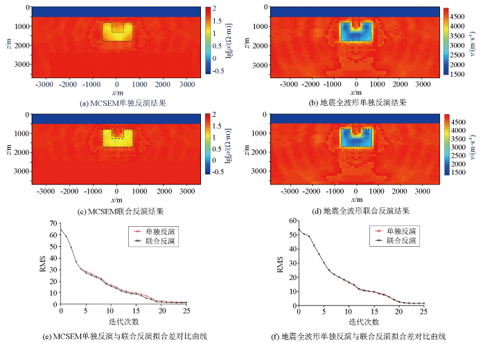
图10
凹槽体模型反演结果及拟合差迭代曲线
Fig.10
The profile of the inversion as well as the iterative curve of the RMS misfit of the groove body model
图10e、f显示在反演过程中两者的RMS值均稳定下降,在后期趋于稳定,其中MCSEM单独反演的RMS值降到1.92,联合反演的RMS值降到1.41左右;地震全波形单独反演与联合反演的RMS曲线基本重合,迭代23次后RMS值稳定在1.51。
4 结论与讨论
1)对MCSEM和地震全波形的二维联合反演理论公式进行了推导,推导出含有交叉梯度项的MCSEM的电阻率迭代公式以及地震全波形的速度迭代公式;建立了基于交叉梯度约束的MCSEM与地震全波形反演的目标函数,开发了一套二维联合反演算法,并验证了该算法的可行性与适用性。
2)建立多组不同的理论模型,进行联合反演计算,并与单一方法反演的结果进行了对比分析。电阻率模型的联合反演结果有显著改善和提升,而速度模型的联合反演结果基本与单方法的结果相同,说明全波形的反演方法能够提高MCSEM反演结果的可靠性。
本文所研究的MCSEM与地震全波形二维联合反演算法并没有加入实际数据的应用,这就使得对于算法精确性的验证具有一定的局限性,下一步需结合实测资料进行正、反演的计算。
参考文献
Joint inversion:A structural approach
[J].DOI:10.1088/0266-5611/13/1/006 URL [本文引用: 1]
2D data-space cross-gradient joint inversion of MT,gravity and magnetic data
[J].DOI:10.1016/j.jappgeo.2017.05.013 URL [本文引用: 1]
Joint inversion of P-wave velocity and density,application to La Soufrière of Guadeloupe hydrothermal system
[J].DOI:10.1111/gji.2012.191.issue-2 URL [本文引用: 1]
地球物理联合反演研究综述
[J].
A review of the researches for geophysical combinative inversion
[J].
Joint electromagnetic and seismic inversion using structural constraints
[J].
DOI:10.1190/1.3246586
URL
[本文引用: 1]

We have developed a frequency-domain joint electromagnetic (EM) and seismic inversion algorithm for reservoir evaluation and exploration applications. EM and seismic data are jointly inverted using a cross-gradient constraint that enforces structural similarity between the conductivity image and the compressional wave (P-wave) velocity image. The inversion algorithm is based on a Gauss-Newton optimization approach. Because of the ill-posed nature of the inverse problem, regularization is used to constrain the solution. The multiplicative regularization technique selects the regularization parameters automatically, improving the robustness of the algorithm. A multifrequency data-weighting scheme prevents the high-frequency data from dominating the inversion process. When the joint-inversion algorithm is applied in integrating marine controlled-source electromagnetic data with surface seismic data for subsea reservoir exploration applications and in integrating crosswell EM and sonic data for reservoir monitoring and evaluation applications, results improve significantly over those obtained from separate EM or seismic inversions.
Using seismic full waveform inversion to constrain controlled-source electromagnetic inversion
[J].
3D constrained inversion of CSEM data with acoustic velocity using full waveform inversion
[C]//
Integrated analysis of CSEM,seismic and well log data for prospect appraisal:A case study from West Africa
[J].
Constrained resistivity inversion using seismic data
[J].DOI:10.1111/gji.2005.160.issue-3 URL [本文引用: 1]
Mixed-grid and staggered-grid finite-difference methods for frequency-domain acoustic wave modelling
[J].DOI:10.1111/gji.2004.157.issue-3 URL [本文引用: 1]
An optimal 9-point,finite-difference,frequency-space,2-D scalar wave extrapolator
[J].
DOI:10.1190/1.1443979
URL
[本文引用: 1]
In this study, a new finite‐difference technique is designed to reduce the number of grid points needed in frequency‐space domain modeling. The new algorithm uses optimal nine‐point operators for the approximation of the Laplacian and the mass acceleration terms. The coefficients can be found by using the steepest descent method so that the best normalized phase curves can be obtained. This method reduces the number of grid points per wavelength to 4 or less, with consequent reductions of computer memory and CPU time that are factors of tens less than those involved in the conventional second‐order approximation formula when a band type solver is used on a scalar machine.
A perfectly matched layer for the absorption of electromagnetic waves
[J].DOI:10.1006/jcph.1994.1159 URL [本文引用: 1]
An overview of full-waveform inversion in exploration geophysics
[J].
DOI:10.1190/1.3238367
URL
[本文引用: 1]
Full-waveform inversion (FWI) is a challenging data-fitting procedure based on full-wavefield modeling to extract quantitative information from seismograms. High-resolution imaging at half the propagated wavelength is expected. Recent advances in high-performance computing and multifold/multicomponent wide-aperture and wide-azimuth acquisitions make 3D acoustic FWI feasible today. Key ingredients of FWI are an efficient forward-modeling engine and a local differential approach, in which the gradient and the Hessian operators are efficiently estimated. Local optimization does not, however, prevent convergence of the misfit function toward local minima because of the limited accuracy of the starting model, the lack of low frequencies, the presence of noise, and the approximate modeling of thewave-physics complexity. Different hierarchical multiscale strategies are designed to mitigate the nonlinearity and ill-posedness of FWI by incorporating progressively shorter wavelengths in the parameter space. Synthetic and real-data case studies address reconstructing various parameters, from [Formula: see text] and [Formula: see text] velocities to density, anisotropy, and attenuation. This review attempts to illuminate the state of the art of FWI. Crucial jumps, however, remain necessary to make it as popular as migration techniques. The challenges can be categorized as (1) building accurate starting models with automatic procedures and/or recording low frequencies, (2) defining new minimization criteria to mitigate the sensitivity of FWI to amplitude errors and increasing the robustness of FWI when multiple parameter classes are estimated, and (3) improving computational efficiency by data-compression techniques to make 3D elastic FWI feasible.
Seismic waveform inversion in the frequency domain,Part 1:Theory and verification in a physical scale model
[J].
DOI:10.1190/1.1444597
URL
[本文引用: 1]
Seismic waveforms contain much information that is ignored under standard processing schemes; seismic waveform inversion seeks to use the full information content of the recorded wavefield. In this paper I present, apply, and evaluate a frequency‐space domain approach to waveform inversion. The method is a local descent algorithm that proceeds from a starting model to refine the model in order to reduce the waveform misfit between observed and model data. The model data are computed using a full‐wave equation, viscoacoustic, frequency‐domain, finite‐difference method. Ray asymptotics are avoided, and higher‐order effects such as diffractions and multiple scattering are accounted for automatically. The theory of frequency‐domain waveform/wavefield inversion can be expressed compactly using a matrix formalism that uses finite‐difference/finite‐element frequency‐domain modeling equations. Expressions for fast, local descent inversion using back‐propagation techniques then follow naturally. Implementation of these methods depends on efficient frequency‐domain forward‐modeling solutions; these are provided by recent developments in numerical forward modeling. The inversion approach resembles prestack, reverse‐time migration but differs in that the problem is formulated in terms of velocity (not reflectivity), and the method is fully iterative. I illustrate the practical application of the frequency‐domain waveform inversion approach using tomographic seismic data from a physical scale model. This allows a full evaluation and verification of the method; results with field data are presented in an accompanying paper. Several critical processes contribute to the success of the method: the estimation of a source signature, the matching of amplitudes between real and synthetic data, the selection of a time window, and the selection of suitable sequence of frequencies in the inversion. An initial model for the inversion of the scale model data is provided using standard traveltime tomographic methods, which provide a robust but low‐resolution image. Twenty‐five iterations of wavefield inversion are applied, using five discrete frequencies at each iteration, moving from low to high frequencies. The final results exhibit the features of the true model at subwavelength scale and account for many of the details of the observed arrivals in the data.
Electromagnetic theory for geophysical applications
[M]//Electromagnetic Methods in Applied Geophysics.
2-D electromagnetic modeling by finite-element method with a dipole source and topography
[J].
DOI:10.1190/1.1444740
URL
[本文引用: 2]
I present a method for calculating frequency‐domain electromagnetic responses caused by a dipole source over a 2-D structure. In modeling controlled‐source electromagnetic data, it is usual to separate the electromagnetic field into a primary (background) and a secondary (scattered) field to avoid a source singularity, and only the secondary field caused by anomalous bodies is computed numerically. However, this conventional scheme is not effective for complex structures lacking a simple background structure. The present modeling method uses a pseudo‐delta function to distribute the dipole source current, and does not need the separation of the primary and the secondary field. In addition, the method employs an isoparametric finite‐element technique to represent realistic topography. Numerical experiments are used to validate the code. Finally, a simulation of a source overprint effect and the response of topography for the long‐offset transient electromagnetic and the controlled‐source magnetotelluric measurements is presented.
An efficient data-subspace inversion method for 2-D magnetotelluric data
[J].
DOI:10.1190/1.1444778
URL
[本文引用: 1]
There are currently three types of algorithms in use for regularized 2-D inversion of magnetotelluric (MT) data. All seek to minimize some functional which penalizes data misfit and model structure. With the most straight‐forward approach (exemplified by OCCAM), the minimization is accomplished using some variant on a linearized Gauss‐Newton approach. A second approach is to use a descent method [e.g., nonlinear conjugate gradients (NLCG)] to avoid the expense of constructing large matrices (e.g., the sensitivity matrix). Finally, approximate methods [e.g., rapid relaxation inversion (RRI)] have been developed which use cheaply computed approximations to the sensitivity matrix to search for a minimum of the penalty functional. Approximate approaches can be very fast, but in practice often fail to converge without significant expert user intervention. On the other hand, the more straightforward methods can be prohibitively expensive to use for even moderate‐size data sets. Here, we present a new and much more efficient variant on the OCCAM scheme. By expressing the solution as a linear combination of rows of the sensitivity matrix smoothed by the model covariance (the “representers”), we transform the linearized inverse problem from the M-dimensional model space to the N-dimensional data space. This method is referred to as DASOCC, the data space OCCAM’s inversion. Since generally N ≪ M, this transformation by itself can result in significant computational saving. More importantly the data space formulation suggests a simple approximate method for constructing the inverse solution. Since MT data are smooth and “redundant,” a subset of the representers is typically sufficient to form the model without significant loss of detail. Computations required for constructing sensitivities and the size of matrices to be inverted can be significantly reduced by this approximation. We refer to this inversion as REBOCC, the reduced basis OCCAM’s inversion. Numerical experiments on synthetic and real data sets with REBOCC, DASOCC, NLCG, RRI, and OCCAM show that REBOCC is faster than both DASOCC and NLCG, which are comparable in speed. All of these methods are significantly faster than OCCAM, but are not competitive with RRI. However, even with a simple synthetic data set, we could not always get RRI to converge to a reasonable solution. The basic idea behind REBOCC should be more broadly applicable, in particular to 3-D MT inversion.
Evidence for correlation of electrical resistivity and seismic velocity in heterogeneous near-surface materials
[J].
Joint two-dimensional DC resistivity and seismic travel time inversion with cross-gradients constraints
[J].
