Correlation tomography is a fast tomography method using correlation coefficients to qualitatively interpret the spatial positions of geobodies. This method, featuring simple, stable, and fast calculations, can quickly and efficiently obtain the distribution of subsurface anomalies without solving large equations. However, the results of direct correlation tomography of gravity anomalies display deep divergence, excessive depth weighting function parameters, and low lateral and vertical resolution between anomalies. According to the fundamental principle of 3D correlation tomography inversion of gravity anomalies, this study introduced the balanced vertical derivative and balanced analytic signal amplitude of gravity anomalies as the edge features to horizontally weight the gravity anomaly correlation tomography, and proposed a more concise depth weighting function. As demonstrated by model tests, the lateral resolution of correlation tomography was improved under the constraint of gravity anomaly edge features, and the vertical resolution of correlation tomography was enhanced using the new depth weighting function. Finally, the method in this study was applied to the actual data of the Australian Olympic Dam polymetallic deposit, yielding consistent weighted tomography results with the actual geological data, thus proving the correctness and effectiveness of the method.
Keywords:gravity anomaly;
correlation tomography;
horizontal weighting;
depth weighting;
edge features
AN Guo-Qiang, LU Bao-Liang, GAO Xin-Yu, ZHU Wu, LI Bo-Sen. 3D correlation tomography inversion of gravity anomalies constrained by edge features and depth weighting[J]. Geophysical and Geochemical Exploration, 2024, 48(1): 113-124 doi:10.11720/wtyht.2024.1053
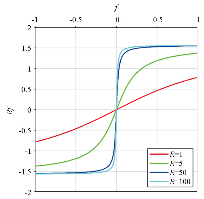
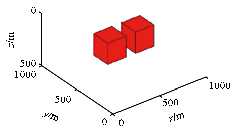
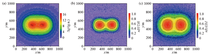
设置两个剩余密度、大小相同的直立长方体模型, 模型参数如表1所示; 平面测网在x、y方向为0~1 000 m, 点距为10 m, 高度位于0 m; 成像范围为0~500 m。 如图4所示, 该模型的重力异常(图4a)含5%高斯白噪声, 计算出该模型的归一化均衡垂向导数(图4b)和归一化均衡解析信号振幅(图4c), 其中均衡系数R=10.0。
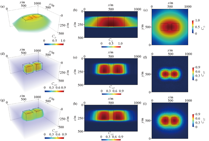
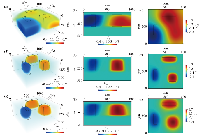
Fig.5
Weighted results of Correlation tomography of two anomalous bodies (including 5% noise) with a residual density of 1.0 g/cm3 and a distance of 100 m
a—imaging results with depth weighted constraints;b—vertical slice at y=500 m(depth weighted constraints);c—horizontal slice at z=200m(depth weighted constraints);d—imaging results of the method in this article (Wz+VDR weighted);e—vertical slice at y=500 m(Wz+VDR weighted);f—Horizontal slice at z=200 m(Wz+VDR weighted);g—imaging results of the method in this article (Wz+ASM weighted);h—vertical slice at y=500 m(Wz+ASM weighted);i—horizontal slice at z=200 m(Wz+ASM weighted)
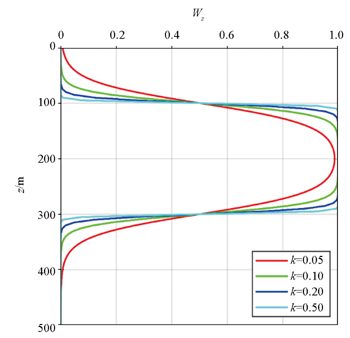
使用本文提出的基于边缘特征与深度加权约束的重力相关成像反演方法的三维结果如图5d、g所示,y=500 m处的垂向切片如图5e、h所示, z=200 m处的水平切片如图5f、i所示。 其中纵向约束使用本文提出的深度加权函数, 先验信息上底z1取100 m, 下底z2取300 m, 调节因子k=0.1。 横向约束分别使用归一化均衡垂向导数和归一化均衡解析信号振幅。 从图中可以看出, 在本文提出的深度加权函数的基础上, 使用归一化均衡垂向导数和归一化均衡解析信号振幅的边缘特征信息均使相关成像的横向分辨率显著提高; 其中, 使用归一化均衡垂向导数的横向分辨率更高。 基于文章篇幅的原因, 本文就不再展示该模型不含噪声的试验。通过对比可知含5%噪声的结果与不含噪声的结果基本相同, 表明相关成像的方法具有良好的抗噪性, 故后文不再展示其他含噪试验结果。
2.2 复杂直立模型试验
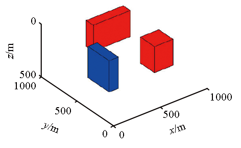
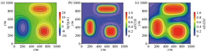
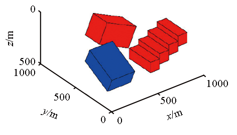
为了研究不同剩余密度成像的效果, 设置了不同剩余密度直立长方体的组合模型; 平面测网在x、y方向为0~1 000 m, 点距为10 m, 高度位于0 m, 成像范围为0~500 m。模型参数如表2所示。该模型的重力异常为图6a, 计算出该模型的归一化均衡垂向导数(图6b)和归一化均衡解析信号振幅(图6c), 其中均衡系数R=2.0。
a—gravity anomaly;b—normalize the balanced vertical derivative (nBVDR);c—normalize the balanced analytical signal amplitude (nBASM)
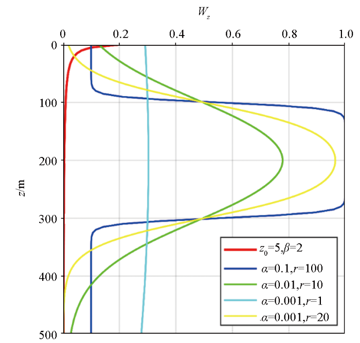
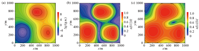
使用Commer等[21]提出的空间梯度加权函数对相关成像进行深度加权。先验深度信息z1=50 m, z2=300 m, 取zmax=500 m, , r=50; 其相关成像深度加权的三维结果如图7a所示, 在水平方向上, 剩余密度为一正一负的异常体之间的边界位置可以区分, 但剩余密度都为正的异常体之间的边界位置无法区分, 横向分辨率很低。
Fig.7
Weighted results of correlation tomography for complex upright model
a—imaging results with depth weighted constraints;b—vertical slice at y=300 m(depth weighted constraints);c—horizontal slice at z=200 m(depth weighted constraints);d—imaging results of the method in this article (Wz+VDR weighted);e—vertical slice at y=300 m(Wz+VDR weighted);f—Horizontal slice at z=200 m(Wz+VDR weighted);g—imaging results of the method in this article (Wz+ASM weighted);h—Vertical slice at y=300 m(Wz+ASM weighted);i—horizontal slice at z=200 m(Wz+ASM weighted)
使用本文方法的三维结果如图7所示, 纵向约束所需先验信息上底z1取50 m, 下底z2取300 m, 调节因子k=0.1。横向约束分别使用归一化均衡垂向导数和归一化均衡解析信号振幅。经过加权后成像的纵向分辨率和横向分辨率显著提高; 其中, 使用归一化均衡垂向导数比归一化均衡解析信号振幅的纵向分辨率更高。
2.3 复杂倾斜模型试验
为了验证更为复杂的情况, 设置了不同剩余密度倾斜长方体和台阶的组合模型; 平面测网在x、y方向为0~1 000 m, 点距为10 m, 高度位于0 m, 成像范围为0~500 m。模型参数如表3所示。该模型的重力异常为图8a, 计算出该模型的归一化均衡垂向导数(图8b)和归一化均衡解析信号振幅(图8c), 其中均衡系数R=10.0。
a—gravity anomaly;b—normalize the balanced vertical derivative (nBVDR);c—normalize the balanced analytical signal amplitude (nBASM)
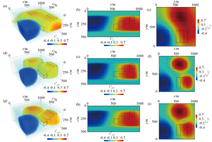
使用Commer等[21]提出的空间梯度加权函数对相关成像进行深度加权三维结果如图9a所示。先验深度信息z1=99 m, z2=430 m, 取zmax=500 m, , r=50; 同样在水平方向上, 剩余密度为一正一负的异常体之间的边界位置可以区分, 但剩余密度都为正的异常体之间的边界位置无法区分, 横向分辨率也很低。使用本文方法的三维结果如图9所示, 纵向约束所需先验信息上底z1取99 m,下底z2取430 m, 调节因子k=0.1。横向约束分别使用归一化均衡垂向导数和归一化均衡解析信号振幅。经过加权后成像的纵向分辨率和横向分辨率显著提高。
Fig.9
Weighted results of correlation tomography for complex tilt model
a—imaging results with depth weighted constraints;b—vertical slice at y=250 m(depth weighted constraints);c—horizontal slice at z=250 m(depth weighted constraints);d—imaging results of the method in this article (Wz+VDR weighted);e—vertical slice at y=250 m(Wz+VDR weighted);f—horizontal slice at z=250 m(Wz+VDR weighted);g—imaging results of the method in this article (Wz+ASM weighted);h—vertical slice at y=250 m(Wz+ASM weighted);i—horizontal slice at z=250 m(Wz+ASM weighted)
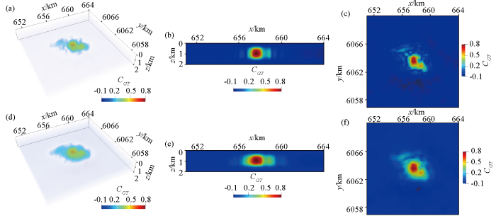
Fig.14
Weighted results of residual gravity anomaly correlation tomography at Olympic Dam, Australia
a—imaging results of the method in this article (Wz+VDR weighted);b—vertical slice at y=6 063.5 km(Wz+VDR weighted);c—horizontal slice at z=750 m(Wz+VDR weighted);d—imaging results of the method in this article (Wz+ASM weighted);e—vertical slice at y=6 063.5 km(Wz+ASM weighted);f—horizontal slice at z=750 m(Wz+ASM weighted)
A new approach to self‐potential (SP) data interpretation for the recognition of a buried causative SP source system is presented. The general model considered is characterized by the presence of primary electric sources or sinks, located within any complex resistivity structure with a flat air‐earth boundary. First, using physical considerations of the nature of the electric potential generated by any arbitrary distribution of primary source charges and the related secondary induced charges over the buried resistivity discontinuity planes, a general formula is derived for the potential and the electric field component along any fixed direction on the ground surface. The total effect is written as a sum of elementary contributions, all of the same simple mathematical form. It is then demonstrated that the total electric power associated with the standing natural electric field component can be written in the space domain as a sum of cross‐correlation integrals between the observed component of the total electric field and the component of the field due to each single constitutive elementary charge. By means of the cross‐correlation bounding inequality, the concept of a scanning function is introduced as the key to the new interpretation procedure. In the space domain, the scanning function is the unit strength electric field component generated by an elementary positive charge. Next, the concept of charge occurrence probability is introduced as a suitable function for the tomographic imaging of the charge distribution geometry underground. This function is defined as the cross‐correlation product of the total observed electric field component and the scanning function, divided by the square root of the product of the respective variances. Using this physical scheme, the tomographic procedure is described. It consists of scanning the section, through any SP survey profile, by the unit strength elementary charge, which is given a regular grid of space coordinates within the section, at each point of which the charge occurrence probability function is calculated. The complete set of calculated grid values can be used to draw contour lines in order to single out the zones of highest probability of concentrations of polarized, primary and secondary electric charges. An extension to the wavenumber domain and to three‐dimensional tomography is also presented and discussed. A few simple synthetic examples are given to demonstrate the resolution power of the new SP inversion procedure.
MaurielloP, PatellaD.
Principles of probability tomography for natural-source electromagnetic induction fields
The 3-D interpretation problem of natural‐source electromagnetic (EM) induction field data collected over a flat air‐earth boundary is dealt with using the concept of probability tomography. This paper presents a method to recognize the most probable localization of the induced electric charge accumulations across resistivity discontinuities and current channeling inside conductive bodies. We begin by writing the solutions for the electric (magnetic) ground surface EM field components in the frequency domain as a sum of elementary contributions, each resulting from a single induced‐charge (dipole) element. Then we express the total electric (magnetic) power associated with each EM field component as a sum of crosscorrelation integrals between the measured component and the homologous synthetic expression resulting from each causative induced‐charge (dipole) element. The synthetic component takes the key role of scanner function in the new imaging procedure. Moreover, using the crosscorrelation bounding inequality we introduce the concept of EM induction occurrence probability as a suitable parameter for the tomographic representation of the induced‐charge and dipole distributions underground. For each electric and magnetic surface component we define the corresponding occurrence probability function as the crosscorrelation product of the observed component and the relative scanning function, divided by the square root of the product of the respective variances. In the space domain, the 3-D tomographic procedure consists of scanning the half‐space below the survey area by the unit strength charge or dipole element, which is given a regular grid of space coordinates within the volume. At each node of the grid, the occurrence probability function is calculated. We use the complete set of calculated grid values to single out the zones of highest occurrence probability of electric charge accumulations and current channeling elements. The physical reliability of the proposed tomography is tested on synthetic and field examples.
MaurielloP, PatellaD.
Gravity probability tomography:A new tool for buried mass distribution imaging
Following the probability tomography principles previously introduced to image the sources of electric and electromagnetic anomalies, we demonstrate that a similar approach can be used to analyse gravity data. First, we give a coherent derivation of the Bouguer anomaly concept as a Newtonian‐type integral for an arbitrary mass distribution buried below a non‐flat topography. A discretized solution of this integral is then derived as a sum of elementary contributions, which are cross‐correlated with the gravity data function in the expression for the total power associated with the Bouguer anomaly. To image the mass distribution underground we introduce a mass contrast occurrence probability function using the cross‐correlation product of the observed Bouguer anomaly and the synthetic field due to an elementary mass contrast source. The tomographic procedure consists of scanning the subsurface with the elementary source and calculating the occurrence probability function at the nodes of a regular grid. The complete set of grid values is used to highlight the zones of highest probability of mass contrast concentrations. Some synthetic and field examples demonstrate the reliability and resolution of the new gravity tomographic approach.
IulianoT, MaurielloP, PatellaD.
Looking inside Mount Vesuvius by potential fields integrated probability tomographies
[J]. Journal of Volcanology and Geothermal Research, 2002, 113(3-4):363-378.
Three-dimensional correlation imaging for total amplitude magnetic anomaly and normalized source strength in the presence of strong remanent magnetization
[J]. Journal of Applied Geophysics, 2014, 111:121-128.
We present a method for inverting surface magnetic data to recover 3-D susceptibility models. To allow the maximum flexibility for the model to represent geologically realistic structures, we discretize the 3-D model region into a set of rectangular cells, each having a constant susceptibility. The number of cells is generally far greater than the number of the data available, and thus we solve an underdetermined problem. Solutions are obtained by minimizing a global objective function composed of the model objective function and data misfit. The algorithm can incorporate a priori information into the model objective function by using one or more appropriate weighting functions. The model for inversion can be either susceptibility or its logarithm. If susceptibility is chosen, a positivity constraint is imposed to reduce the nonuniqueness and to maintain physical realizability. Our algorithm assumes that there is no remanent magnetization and that the magnetic data are produced by induced magnetization only. All minimizations are carried out with a subspace approach where only a small number of search vectors is used at each iteration. This obviates the need to solve a large system of equations directly, and hence earth models with many cells can be solved on a deskside workstation. The algorithm is tested on synthetic examples and on a field data set.
CommerM, NewmanG A, WilliamsK H, et al.
3D induced-polarization data inversion for complex resistivity
The conductive and capacitive material properties of the subsurface can be quantified through the frequency-dependent complex resistivity. However, the routine three-dimensional (3D) interpretation of voluminous induced polarization (IP) data sets still poses a challenge due to large computational demands and solution nonuniqueness. We have developed a flexible methodology for 3D (spectral) IP data inversion. Our inversion algorithm is adapted from a frequency-domain electromagnetic (EM) inversion method primarily developed for large-scale hydrocarbon and geothermal energy exploration purposes. The method has proven to be efficient by implementing the nonlinear conjugate gradient method with hierarchical parallelism and by using an optimal finite-difference forward modeling mesh design scheme. The method allows for a large range of survey scales, providing a tool for both exploration and environmental applications. We experimented with an image focusing technique to improve the poor depth resolution of surface data sets with small survey spreads. The algorithm’s underlying forward modeling operator properly accounts for EM coupling effects; thus, traditionally used EM coupling correction procedures are not needed. The methodology was applied to both synthetic and field data. We tested the benefit of directly inverting EM coupling contaminated data using a synthetic large-scale exploration data set. Afterward, we further tested the monitoring capability of our method by inverting time-lapse data from an environmental remediation experiment near Rifle, Colorado. Similar trends observed in both our solution and another 2D inversion were in accordance with previous findings about the IP effects due to subsurface microbial activity.
HoodP, McClureD J.
Gradient measurements in ground magnetic prospecting
The total magnetic field values over an area can be represented exactly by a double Fourier series expansion. In this analysis, such an expansion is used to evaluate very accurately the fields continued downward and upward from the plane of observation and the vertical derivatives of the total field. This harmonic expansion of the anomalous total field makes it possible to calculate, with exceptional accuracy, the field reduced to the magnetic pole and its second derivative. The results of the calculations are free from the effect of the inclination of the earth’s main geomagnetic field and that of the polarization vector, at all magnetic latitudes and for all possible directions of polarization. In order to determine the influence of remanence on the above field, a number of anomalies caused by rectangular block‐type bodies with known polarization are reduced to the magnetic pole, correcting only for the obliquity of the earth’s normal field. It is concluded from a study of these anomalies that the interpretation of magnetic data based on the assumption of rock magnetization due solely to induction in the earth’s field may yield erroneous results, particularly when remanence is important.
NabighianM N.
The analytic signal of two-dimensional magnetic bodies with polygonal cross-section:Its properties and use for automated anomaly interpretation
This paper presents a procedure to resolve magnetic anomalies due to two‐dimensional structures. The method assumes that all causative bodies have uniform magnetization and a cross‐section which can be represented by a polygon of either finite or infinite depth extent. The horizontal derivative of the field profile transforms the magnetization effect of these bodies of polygonal cross‐section into the equivalent of thin magnetized sheets situated along the perimeter of the causative bodies. A simple transformation in the frequency domain yields an analytic function whose real part is the horizontal derivative of the field profile and whose imaginary part is the vertical derivative of the field profile. The latter can also be recognized as the Hilbert transform of the former. The procedure yields a fast and accurate way of computing the vertical derivative from a, given profile. For the case of a single sheet, the amplitude of the analytic function can be represented by a symmetrical function maximizing exactly over the top of the sheet. For the case of bodies with polygonal cross‐section, such symmetrical amplitude functions can be recognized over each corner of each polygon. Reduction to the pole, if desired, can be accomplished by a simple integration of the analytic function, without any cumbersome transformations. Narrow dikes and thin flat sheets, of thickness less than depth, where the equivalent magnetic sheets are close together, are treated in the same fashion using the field intensity as input data, rather than the horizontal derivative. The method can be adapted straightforwardly for computer treatment.It is also shown that the analytic signal can be interpreted to represent a complex “field intensity,” derivable by differentiation from a complex “potential.” This function has simple poles at each polygon corner. Finally, the Fourier spectrum due to finite or infinite thin sheets and steps is given in the Appendix.
NabighianM N.
Toward a three-dimensional automatic interpretation of potential field data via generalized Hilbert transforms:Fundamental relations
The paper extends to three dimensions (3-D) the two‐dimensional (2-D) Hilbert transform relations between potential field components. For the 3-D case, it is shown that the Hilbert transform is composed of two parts, with one part acting on the X component and one part on the Y component. As for the previously developed 2-D case, it is shown that in 3-D the vertical and horizontal derivatives are the Hilbert transforms of each other. The 2-D Cauchy‐Riemann relations between a potential function and its Hilbert transform are generalized for the 3-D case. Finally, the previously developed concept of analytic signal in 2-D can be extended to 3-D as a first step toward the development of an automatic interpretation technique for potential field data.
VellaL.
Interpretation and modelling,based on petrophysical measurements,of the wirrda well potential field anomaly,South Australia
Gravity inversion is inherently nonunique. Minimum-structure inversion has proved effective at dealing with this non-uniqueness. However, such an inversion approach, which involves a large number of unknown parameters, is computationally expensive. To improve efficiency while retaining the advantages of a minimum-structure-style inversion, we have developed a new method, based on edge detection and center detection of geologic bodies, to help to focus the spatial extent of meshing for gravity inversion. The chosen method of edge detection, normalized vertical derivative of the total horizontal derivative, helps to outline areas to be meshed by approximating the edges of key geophysical bodies. Next, the method of center detection, normalized vertical derivative of the analytic signal amplitude, helps to confirm the center of the areas to be meshed, then a binary mesh flag is generated. In this paper, the binary mesh flag, restricting the spatial extent of meshing, is first undertaken using the two methods, and it is shown to dramatically reduce the number of grid cells from 574,992 for the whole research volume to 170,544 for the localized mesh by the same size of cell, which is decreased by almost 70%. Second, gravity inversion is performed using the spatially restricted mesh. The recovered model constructed using the binary mesh flag is similar to the model obtained using the mesh spanning the whole volume and saves approximately 80% of the CPU time. Finally, a real gravity data example from Olympic Dam in Australia is successfully used to test the validity and practicability of this proposed method. The geologic source bodies are resolved between 250 and 750 m depth. Overall, the combination of edge detection and center detection, and our binary mesh flag, succeed in reducing the number of cells and saving the CPU time and computer storage required for gravity inversion.
ZhangS, YinC C, CaoX Y, et al.
DecNet:Decomposition network for 3D gravity inversion
Three dimensional gravity inversion is an effective way to extract subsurface density distribution from gravity data. Different from the conventional geophysics-based inversions, machine-learning-based inversion is a data-driven method mapping the observed data to a 3D model. We have developed a new machine-learning-based inversion method by establishing a decomposition network (DecNet). Unlike existing machine-learning-based inversion methods, the proposed DecNet method is a mapping from 2D to 2D, which requires less training time and memory space. Instead of learning the density information of each grid point, this network learns the boundary position, vertical center, thickness, and density distribution by 2D-to-2D mapping and reconstructs the 3D model by using these predicted parameters. Furthermore, by using the highly accurate boundary information learned from this network as supplement information, the DecNet method is optimized into a DecNetB method. By comparing the least-squares inversion and U-Net inversion on synthetic and real survey data, the DecNet and DecNetB methods have shown the advantage in dealing with inverse problems for targets with boundaries.
Introduction to ground surface self-potential tomography
Three-dimensional correlation imaging for total amplitude magnetic anomaly and normalized source strength in the presence of strong remanent magnetization
... 使用Commer等[21]提出的空间梯度加权函数对相关成像进行深度加权.先验深度信息z1=50 m, z2=300 m, 取zmax=500 m, , r=50; 其相关成像深度加权的三维结果如图7a所示, 在水平方向上, 剩余密度为一正一负的异常体之间的边界位置可以区分, 但剩余密度都为正的异常体之间的边界位置无法区分, 横向分辨率很低. ...
... 使用Commer等[21]提出的空间梯度加权函数对相关成像进行深度加权三维结果如图9a所示.先验深度信息z1=99 m, z2=430 m, 取zmax=500 m, , r=50; 同样在水平方向上, 剩余密度为一正一负的异常体之间的边界位置可以区分, 但剩余密度都为正的异常体之间的边界位置无法区分, 横向分辨率也很低.使用本文方法的三维结果如图9所示, 纵向约束所需先验信息上底z1取99 m,下底z2取430 m, 调节因子k=0.1.横向约束分别使用归一化均衡垂向导数和归一化均衡解析信号振幅.经过加权后成像的纵向分辨率和横向分辨率显著提高. ...
Gradient measurements in ground magnetic prospecting
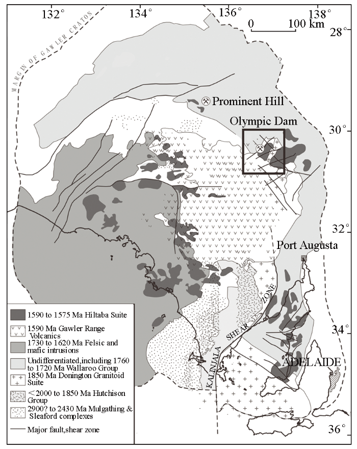
... [35]Basement geological map of the Gawler Craton Province <sup>[<xref ref-type="bibr" rid="b35">35</xref>]</sup>Fig.1010.11720/wtyht.2024.1053.F0011
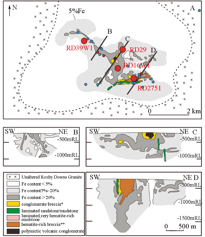
Simplified geological map and cross-sectional subsurface structure of the supergiant Olympic Dam breccia complex <sup>[<xref ref-type="bibr" rid="b36">36</xref>]</sup>Fig.1110.11720/wtyht.2024.1053.F0012
Simplified geological map and cross-sectional subsurface structure of the supergiant Olympic Dam breccia complex <sup>[<xref ref-type="bibr" rid="b36">36</xref>]</sup>Fig.1110.11720/wtyht.2024.1053.F0012
... [36]Simplified geological map and cross-sectional subsurface structure of the supergiant Olympic Dam breccia complex <sup>[<xref ref-type="bibr" rid="b36">36</xref>]</sup>Fig.1110.11720/wtyht.2024.1053.F0012


