

0 引言
大地电磁测深是一种以天然电磁场为场源的地球物理勘探方法,其观测频带较宽,有效信号微弱,随着人文噪声的日益增加,大地电磁的“净土”已经基本消失。其中,由测区附近用电设备的充放电所引起的方波噪声是一种常见的高强度噪声,主要集中在电道,可产生高于正常信号十几倍到几十倍的干扰[1-2],这类噪声影响幅度大,影响频点多,极大干扰了阻抗估计的结果。为了压制方波干扰,许多学者做了大量研究:严家斌[3]提出了基于小波变换的迭代回归噪声改正方法,对含方波干扰的脉冲类噪声进行了压制,有效改善了数据质量;蔡建华等[4]将经验模态分解(EMD)应用于方波噪声处理,突出了有用信号;汤井田、李晋等[5]提出了一种基于数学形态滤波的大地电磁去噪方法,对安徽庐枞矿集区的方波、脉冲、三角波等噪声进行了处理,有效抑制了大尺度干扰和基线漂移;汤井田、刘祥等[6]讨论了不同仿真方波噪声对测深曲线的影响及远参考法对其的去噪效果,研究表明远参考在一定条件下可以消除方波干扰;王辉、魏文博等[7]利用同步大地电磁时间序列信号之间的关系,用合成的无噪数据段代替含噪数据段,成功去除了大于窗口长度的方波噪声,精度较高,但该方法需要一段无明显干扰的远参考数据;汤井田、李广等[8]通过字典学习提取人文干扰特征,利用构建的冗余字典分离了AMT数据中的仿真方波噪声;李晋、张贤等[9]利用变分模态分解(VMD)和匹配追踪(MP)对模拟方波噪声进行了处理,明显改善了数据质量。
近年来,深度学习已经在地球物理部分方法的应用中取得了不错的效果[10],不少学者将其成功引入电磁、地震数据处理以及重磁反演等地球物理领域[11-15]。深度学习方法适用范围广,泛化能力强,在大地电磁方面的应用主要集中在时间序列处理上,Manoj和Nagarajan[16]最早提出了利用人工神经网络自动执行大地电磁时间序列编辑的方法,该方法提高了工作效率减少了人工编辑的主观因素。本文所应用的长短时记忆网络(long short-term memory, LSTM)是一种特殊的循环神经网络,该神经网络在语音识别、自然语言处理以及时间序列相关的领域有较为广泛的应用,近年来也被逐渐引入到地球物理领域,例如:许滔滔等[17]将LSTM网络应用于工频干扰压制,有效去除了工频干扰;王斯昊等[18]用LSTM网络去除了时间序列的阶跃信号;汪凯翔等[19]利用LSTM网络对地电场数据进行了处理,去除了测试集中不同种类的噪声。以上方法都是以时间序列的低频、大尺度噪声或者信号轮廓为网络输出值。与前人不同的是,本文使用大地电磁信号本身作为网络输出,通过选取标准大地电磁时间序列随机添加仿真方波噪声作为网络训练输入,以无噪大地电磁时间序列作为网络目标输出,让网络存储和学习大地电磁信号本身的特征,从含噪时间序列中自动提取符合大地电磁信号特征的序列,从而实现抑制方波噪声的目的。
1 LSTM网络简介
长短时记忆网络(LSTM)是一种特殊的循环神经网络,由Hochreiter和Schmidhuber于1997年提出[20],主要是为了解决长序列训练过程中的梯度消失和梯度爆炸问题,被广泛应用于时间序列相关领域。
一个标准的LSTM网络神经元包含了3个门(输入门、输出门、遗忘门)和1个记忆细胞(图1),可以归纳为以下几式:
式中:ht-1为t-1时刻即上一个神经元的隐藏层;xt为t时刻的特征向量;σ为sigmoid激活函数;it、ft、ot分别为t时刻输入门、遗忘门和输出门的状态;gt为t时刻记忆细胞的候选值;ct为t时刻记忆细胞的状态,也作为t+1时刻即下一个神经元的初始记忆细胞;ht为t时刻的隐藏层,也为t+1时刻即下一个神经元的初始隐藏层;Wi、Wf、Wo、Wg为传播权重矩阵;bi、bf、bo、bg为偏置向量;☉表示矩阵元素对应相乘。
图1
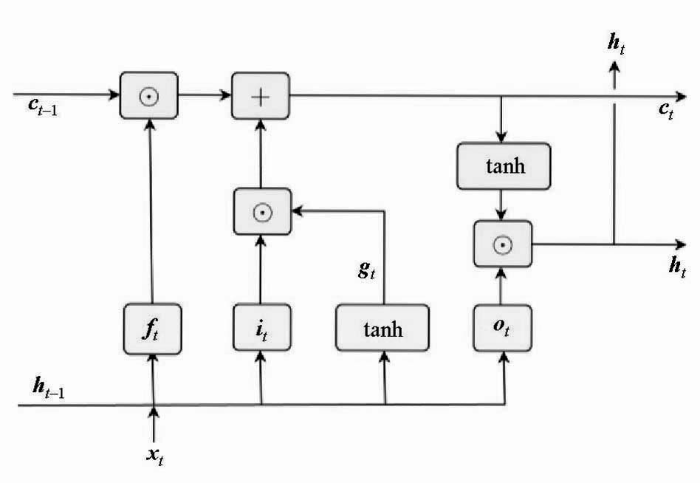
总的来说,单向LSTM神经元内部有3个处理步骤:
第一步为选择忘记阶段,主要是对上一个节点传进来的输入进行选择性忘记。根据上一个神经元所传递的隐藏层ht-1和本神经元的输入xt生成遗忘门ft,来控制上一个神经元所传递的记忆细胞ct-1中哪些需要留,哪些需要“忘”(式(1)、式(5))。
第二步为选择记忆阶段,主要是通过上一个神经元的隐藏层和本次的输入xt生成输入门it,再与t时刻记忆细胞的候选值gt作用来决定需要记住的信息(式(2)、式(4)、式(5))。
第三部为输出阶段。通过前两个阶段的“遗忘”和“记忆”,共同决定了记忆细胞ct的最新状态,而后ct通过激活函数tanh的放缩,由输出门ot控制生成新的隐藏层状态ht(式(4)、式(5)、式(6))。
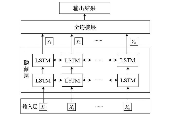
本文使用双向LSTM网络。双向LSTM网络就是在序列正向处理的基础上将序列逆向再处理一次,这样神经元不仅能获取“过去”时刻的序列信息,也能获取“未来”时刻的信息,能更好地记录其上下文的关系,从而取得更佳的学习效果。
2 LSTM网络搭建
2.1 网络设计
图2
2.2 网络训练
网络训练主要包括数据集构建、数据集归一化(或标准化)、网络训练和验证等几个步骤。
2.2.1 数据集构建
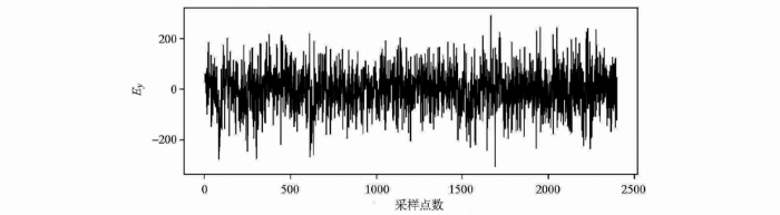
选取2020年10月12日在陕西省宁强县某地用MTU-5A大地电磁仪采集的、无明显人文干扰且阻抗估计稳定的数据段Ex通道序列,将其视为无噪声的大地电磁时间序列,长度2 400个点,采样率2 400 Hz(图3)。首先,随机生成100组方波信号,因为待处理的实测方波噪声主频在24 Hz左右,故模拟方波噪声频率随机分布在23~25 Hz之间,振幅在该段无噪时间序列最大值与最小值之差的0.1~8倍之间随机取值,相位随机。而后,将所有模拟方波噪声各自叠加在无噪大地电磁时间序列上,合成100组仿真含噪信号,并在每组仿真信号中随机截取64组长度 1 200个点的信号,共产生6 400组信号作为训练集;选取与训练集Ex对应的Ey通道数据,长度2 400个点,采样率2 400 Hz(图4),将该段数据采用与合成训练集同样的方式生成20组仿真含方波噪声时间序列,而后每组信号随机截取64组长度为1 200个点的信号,共1 280组信号作为验证集,以验证网络的实际处理能力。
图3
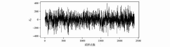
图4
2.2.2 数据归一化
数据集构建好后还要进行数据归一化(或标准化),归一化后数据可以提高网络的收敛速度和网络精度,根据大地电磁时间序列数据的特征,将其归一化至1~-1之间。
对于网络输入数据:
式中:x为添加模拟噪声的大地电磁时间序列数据,xmean为其平均值,xmax为其最大值,xnorm为归一化值。
对于网络的目标输出数据:
式中:y为不含噪声的大地电磁时间序列数据,xmax为含噪数据的最大值,ynorm为归一化值。
对所有输入网络的数据都要进行归一化,包括训练集、验证集,由于网络的理想输出为归一化值,输出后还要进行反归一化:
式中:ypred为反归一化值,即为实际无噪大地电磁数据;ynorm_pred为网络输出的归一化预测值;xmax为网络输入的含噪大地电磁信号的最大值。
2.2.3 网络的训练和验证
将bitch_size(一次训练所选取的样本数)设为32,epoch(使用训练集中的全部样本训练一次即为1个epoch)数设置为3 000,以保证网络的收敛。
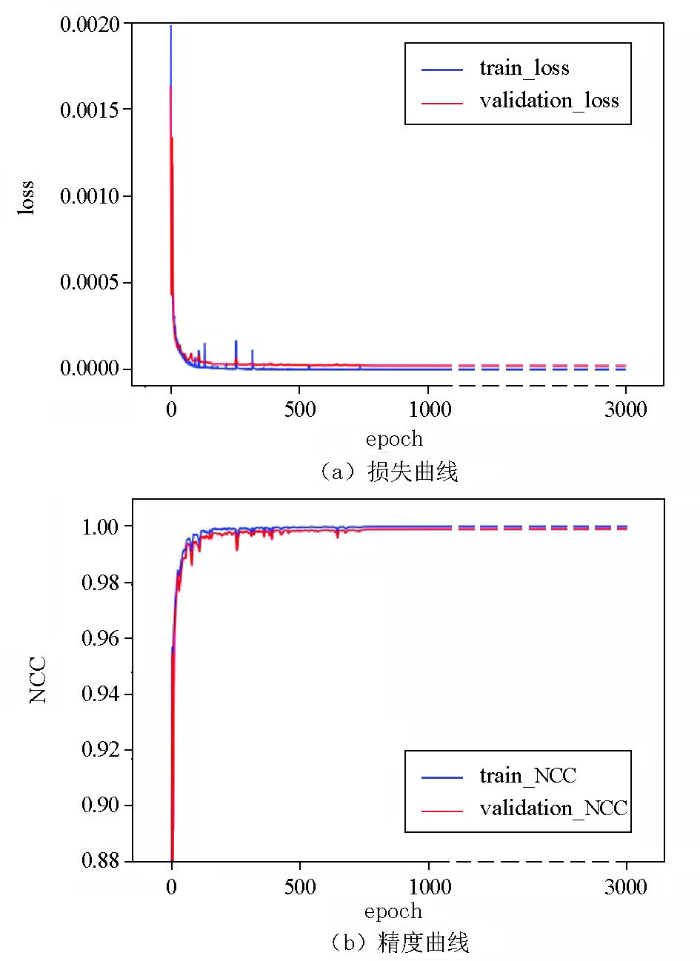
评价网络训练效果的主要有网络损失曲线和网络精度曲线。本文选取网络理想输出时间序列和实际输出时间序列的归一化互相关系数(normalized cross correlation,NCC)作为检验网络精度的参数,具体计算如下:
由LSTM网络的学习曲线(图5)可知,前500次epoch损失曲线急剧下降,精度曲线快速上升;训练500次以后损失曲线缓慢下降,精度曲线缓慢上升,训练集损失(train_loss)略小于验证集(validation_loss),训练集精度(train_NCC)略大于验证集(validation_NCC)。当训练至1 500次epoch时,训练集的平均NCC可达0.999 98,验证集的平均NCC可达0.999 03,说明网络很好地从含方波噪声的序列中提取出了有效大地电磁时间序列。训练1 500次以后网络趋于稳定,验证集损失几乎不再减小,精度不再明显增加,故取epoch为1 500的网络为最终模型,用来进行下一步去噪测试。
图5
3 去噪测试
3.1 仿真含噪信号去噪
选取陕西省宁强县某地2020年10月16日使用MTU-5A大地电磁仪所采集的无明显人文干扰且阻抗估计稳定的Ex通道时间序列数据段作为测试信号,数据长24 000个点,采样率2 400 Hz,由于数据过长故截取其中1 s(2 400个点)进行展示(图6)。给测试信号叠加一主频24 Hz,振幅为该段测试信号最大值与最小值之差1.5倍的方波噪声作为仿真含噪信号(图6c),用训练好的LSTM网络进行去噪试验。由于天然大地电磁信号的复杂性,在实际使用LSTM网络提取一次大地电磁信号后,残余噪声里还含有部分低频有效信号,可以使用网络进行多次提取,一定程度上可以减小信号损失,但同时也会引入更多的噪声,应该具体情况具体分析。本文所有去噪均为网络提取一次的结果。
图6
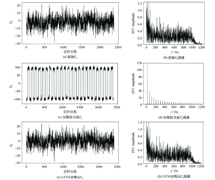
图6
仿真信号片段去噪前后对比
Fig.6
Comparison of Simulation signal fragment before and after denoising
图7
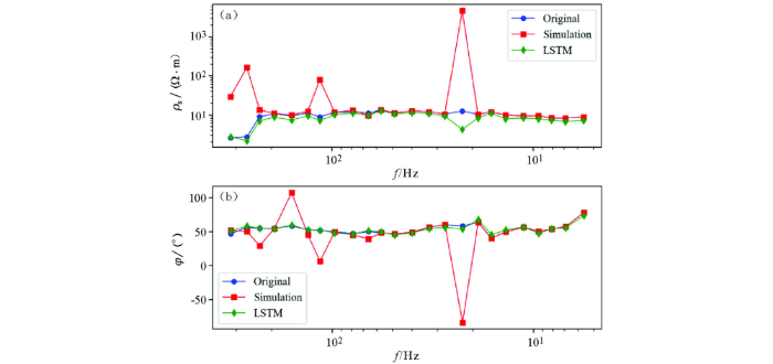
图7
仿真信号去噪前后电阻率、阻抗结果对比
Fig.7
Comparison of resistivity and impedance before and after denoising of simulated signals
3.2 实测含噪信号去噪
图8
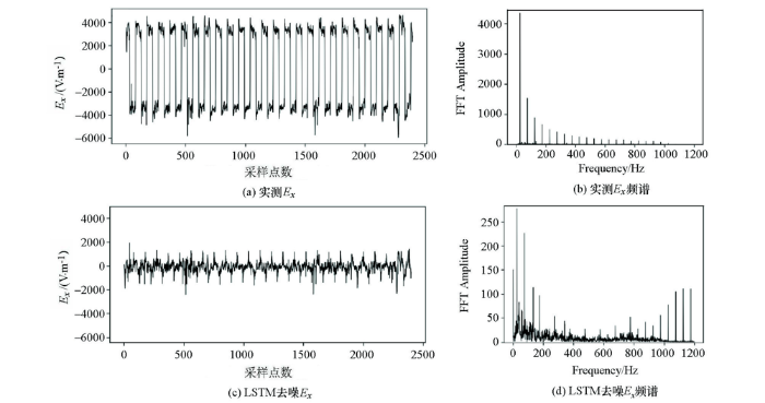
图9
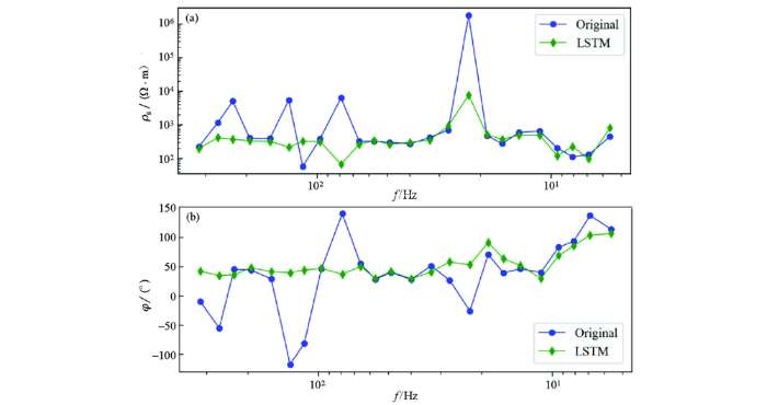
图9
实测信号去噪前后电阻率、阻抗对比
Fig.9
Comparison of resistivity and impedance before and after denoising of measured signals
为了进一步评价实测信号去噪效果在此引入奈奎斯特图[22-23],在无噪声干扰条件下,大地电磁阻抗的奈奎斯特图是从低频到高频呈顺时针展布的连续光滑曲线,一旦某个频点受到干扰该频点将会脱离这种趋势,所以可以根据奈奎斯特图是否更具有这种趋势来评判去噪效果。去噪前,实测信号阻抗的奈奎斯特图特征比较混乱,特别是在22.5 Hz、79 Hz、132 Hz、229 Hz等频点处严重脱节,几乎无法识别出其顺时针旋转特征(图10a)。经本文方法去噪后,除22.5 Hz较其他频点偏离较大之外,其余频点虽然也不是光滑连续分布,但是基本滤除了大尺度方波对阻抗的干扰,奈奎斯特图总体趋势基本符合从低频到高频顺时针展布的特征(图10b),与去噪前相比阻抗结果更加稳定和合理。
图10
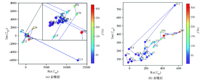
图10
实测信号去噪前后的奈奎斯特图对比
Fig.10
Comparison of Nyquist diagrams before and after denoising of measured signals
4 结论与建议
与前人将噪声作为LSTM网络的期望输出不同的是,本文采用大地电磁信号本身作为网络期望输出,用训练好的网络进行了仿真含方波噪声和实测含方波噪声的大地电磁时间序列去噪测试,结果表明本文所提方法能有效消除方波噪声干扰,改善阻抗估计结果,为深度学习在大地电磁时间序列去噪领域的应用提出了新思路。
致谢
感谢中国地质调查局西安矿产资源调查中心郝子琼对本文网络训练的支持!
参考文献
大地电磁测深资料的噪声干扰
[J].
Noise interference of magnetotelluric data
[J].
庐枞矿集区大地电磁测深强噪声的影响规律
[J].
Effect rules of strong noise on magnetotelluric (MT) sounding in Luzong ore cluster area
[J].
基于经验模态分解的大地电磁资料人文噪声处理
[J].
Human noise elimination for magnetotelluric data based on empirical mode decomposition
[J].
数学形态滤波与大地电磁噪声压制
[J].
Mathematical morphology filtering and noise suppression of magnetotelluric sounding data
[J].
仿真方波的大地电磁远参考去噪研究
[J].
Simulation of square waveform de-noising research of magnetotelluric with a remote reference
[J].
基于同步大地电磁时间序列依赖关系的噪声处理
[J].
Removal of magnetotelluric noise based on synchronous time series relationship
[J].
基于字典学习的音频大地电磁数据处理
[J].
Denoising AMT data based on dictionary learning
[J].
利用变分模态分解(VMD)和匹配追踪(MP)联合压制音频大地电磁(AMT)强干扰
[J].
Suppression of strong interference for AMT using VMD and MP
[J].
深度学习在地球物理中的应用现状与前景
[J].
Current status and application prospect of deep learning in geophysics
[J].
基于在线惯序极限学习机的瞬变电磁非线性反演
[J].
Online sequential extreme learning machine for transient electromagnetic nonlinear inversion
[J].
基于卷积神经网络识别重力异常体
[J].
The identification of gravity anomaly body based on the convolutional neural network
[J].
基于深度学习卷积神经网络的地震数据随机噪声去除
[J].
Deep learning convolutional neural networks for random noise attenuation in seismic data
[J].
大地电磁人工神经网络反演
[J].
Magnetotelluric inversion using artificial neural network
[J].
BP神经网络磁性体顶面埋深预测方法
[J].
Prediction of magnetic body top based on BP neural network
[J].
The application of artificial neural networks to magnetotelluric time-series analysis
[J].
基于LSTM 循环神经网络的大地电磁工频干扰压制
[J].
Magnetotelluric power frequency interference suppression based on LSTM recurrent neural network
[J].
基于LSTM循环神经网络的MT时间序列去噪可行性分析
[C]//
Feasibility analysis of the LSTM based denoising to MT time series
[C]//
长短时记忆神经网络在地电场数据处理中的应用
[J].
Application of long short-term memory neural network in geoelectric field data processing
[J].
Long short-term memory
[J].Learning to store information over extended time intervals by recurrent backpropagation takes a very long time, mostly because of insufficient, decaying error backflow. We briefly review Hochreiter's (1991) analysis of this problem, then address it by introducing a novel, efficient, gradient-based method called long short-term memory (LSTM). Truncating the gradient where this does not do harm, LSTM can learn to bridge minimal time lags in excess of 1000 discrete-time steps by enforcing constant error flow through constant error carousels within special units. Multiplicative gate units learn to open and close access to the constant error flow. LSTM is local in space and time; its computational complexity per time step and weight is O(1). Our experiments with artificial data involve local, distributed, real-valued, and noisy pattern representations. In comparisons with real-time recurrent learning, back propagation through time, recurrent cascade correlation, Elman nets, and neural sequence chunking, LSTM leads to many more successful runs, and learns much faster. LSTM also solves complex, artificial long-time-lag tasks that have never been solved by previous recurrent network algorithms.
Adam:A method for stochastic optimization
[J].
Imaging strategies to interpret 3-D noisy audio-magnetotelluric data acquired in Gyeongju South Korea:data processing and inversion
[J].DOI:10.1093/gji/ggab002 URL [本文引用: 1]
Magnetotelluric transfer function distortion assessment using Nyquist diagrams
[J].
DOI:10.1016/j.jappgeo.2018.11.018
[本文引用: 1]

Magnetotelluric (MT) inversion is using impedance data as input data, which is traditionally presented via the apparent resistivity and impedance phase. Since high-quality MT data are necessary to improve the reliability of inversion results, the distortions in the curves should be assessed and removed. Usually, this smoothing procedure acts individually on the apparent resistivity and phase and does not consider the dispersion relationship between the real and imaginary parts of the impedance. Therefore, how to assess the distortion while retaining the inherent relationship in the impedance should be addressed. In this study, Nyquist diagrams were used as a tool to illustrate the inherent feature of the MT complex response. The MT impedances of 2-D and 3-D models were computed and illustrated in the corresponding diagrams. From these curves, we found that the Nyquist curves or part of them are continuous and smooth. When the model is 1-D or 2-D, Z(xy) and Z(yx) try to stretch around a line at a 45 degrees slope, whereas in the 3-D case, the Nyquist diagrams of the full impedance elements rotate clockwise from low to high frequencies. If the frequency is high or low enough, the curves of Z(xx) and Z(yy) become approximate ellipses. The phases of Z(xx) and z(yy) are also out of scope (-pi,pi), which is beyond the traditional knowledge of the phase, which making data distortion removal in the phase confusing. Cole-Cole model could be used to explain above features. And these features behind the Nyquist diagrams could be used as tools to guide the distortion removal in the MT complex response in the field. When MT impedance data are not severely distorted, it is possible to recover high-quality data when obeying the following two rules: (1) both the amplitude and phase should be smooth and (2) the Nyquist curve of the complex response should also be smooth or at least smooth in segments. (C) 2018 Published by Elsevier B.V.
大地电磁信号统计特征分析
[J].
Analysis on statistic characteristics of Magnetotelluric signal
[J].
Nonstationary magnetotelluric data processing with instantaneous parameter
[J].DOI:10.1002/2013JB010494 URL [本文引用: 1]
