

0 引言
重力勘探在油气与矿产资源勘查、地质填图、考古探测、工程与环境等地质学科中发挥着重要作用。随着测量手段的多样化和测量数据精度的提高,欲在一定精度的数据基础上,达到理想的处理和解释效果,则需要与数据相对应的新方法与新技术。因此,新的处理和解释方法是地球物理学者长期以来一直致力于探索和研究的重要问题。伴随着全(或部分)重力梯度张量数据越来越多地应用于各个领域,其处理和解释的方法和技术研究也己经成为新的重要课题。
快速成像法是相对于传统常规反演方法而提出的[1,2,3],由于不需要任何的迭代过程,因此能够快速地得到地下异常体的分布状况或相关参量(如深度、倾角及构造指数等),避免了传统方法耗时长、计算量大等缺陷。Fedi和Pilkington于2012年总结并比较了位场成像方法[4],包括Cribb[5]于1976年提出的Cribb成像法、Moreau等[6]于1999年阐述的连续小波变换法、Mauriello等[7]于2001年提出的概率成像法、Zhdanov等[8]在2011年提出的偏移成像法以及Fedi[9]于2007年提出的极值点深度估计法(DEXP)等。为了将这些方法应用于重力梯度张量数据解释,国内外学者们将许多方法均进行了一定程度的改进(如Guo等[10]; Zhdanov等[11]; Zhou等[12])。
DEXP方法是一种重要的成像方法,该方法由Fedi在2007年提出并对其进行了详细的阐述[9],由于在计算过程中深度加权函数引入了构造指数,使得与其他方法相比具有许多优点。该方法的适用性比较广,不仅可以用于重力异常不同阶次导数以估计异常体的物性参数[9](如场源深度、剩余密度及构造指数等),同时也是一种解释自然电位数据的可靠方法[13]。Abbas等[14]又在2014年提出了一种利用两个不同阶导数场之间的比值解释位场数据的自动DEXP方法,该方法在成像过程中不依赖于异常体的构造指数。此外,DEXP方法还可以与其他方法结合使用(Fedi等[15])。之后,Zhou等[12]又进一步将DEXP成像法用于重力梯度张量数据处理中,取得了较好的成像结果。笔者根据DEXP变换理论,通过设置多组理论模型及其模拟数据进行试验研究,结合实际应用,着重讨论了DEXP成像方法的抗噪能力以及数据的点距、计算范围和背景场对DEXP变换结果的影响。
1 方法原理
对于可视作质点或均匀球体的重力异常为:
其中:G为万有引力常数(G=6.67×10⁻¹¹ m3·kg-1·s-2),r为坐标原点指向测量点P(x, y, z)的矢量,r0为坐标原点指向质点或球心Q(x0,y0,z0)的矢量。在笛卡尔直角坐标系下,假设质心或球心的位置为(0,0,z0),测量点的水平位置为x=x0=0、y=y0=0以及z>0,令质量M=1,并且将万有引力常数进行归一化处理,则式(1)可简化为:
进一步地,式(2)的任意p阶导数fp可以写为:
其中:z0为场源的中心埋深,Np为重力异常p阶垂向导数对应的构造指数,定义为Np=N+p。其中N为构造指数,是与场源几何形态相关的参数[16]。
根据式(4),Fedi[9]将重力异常p阶垂向导数的DEXP变换函数Wp定义为:
并且证明了DEXP变换函数的极值点可用于估算场源深度。
重力梯度张量的各个元素为重力位U在笛卡尔直角坐标系下三个坐标轴方向的二阶导数,即
将式(6)写成矩阵形式,即:
由于重力异常位在场源外部空间满足拉普拉斯方程,即Δ2U(r)=Txx+Tyy+Tzz=0,并且矩阵T为对称矩阵,故重力梯度张量仅有5个独立元素。
对于重力梯度数据,不同分量反映了地下异常体的不同特征信息,比如Txz、Tyz主要反映的是异常体的边界信息,而Tzz则可以描述场源中心位置信息。因此,重力梯度张量的DEXP变换也具有相似的特征。Zhou[12]指出Wxx、Wyy和Wzz可以用来描述地下异常体的中心埋深、Wxz和Wyz则可以根据不同极值点深度位置确定场源的边界信息,同时也指出DEXP变换的总水平导数Wthd能够反映异常体的总体边界信息,其计算公式为:
2 基于理论模型的影响因素分析
首先令均匀直立棱柱体模型的长(a)、宽(b)与高(c)分别为30、20与10 m,其中心埋深为15 m,剩余密度Δρ为0.5 g/cm3。首先, 通过正演计算可以得到该模型在地表即z=0处产生的重力异常以及重力梯度张量异常;其次,分别将模拟数据在波数域进行不同高度的向上延拓处理以得到3D数据体;然后,根据DEXP变换理论,分别可得模型重力异常以及重力梯度张量异常的DEXP变换结果,分别如图1与图2所示。其中,模拟数据的测点点距为2 m,向上延拓总高度为40 m,步长为1 m。图中黑色矩形描述了直立棱柱体模型的边界位置,白色实线为DEXP变换后所选取的剖面位置,白色圆点为DEXP变换对应的极值点。
图1
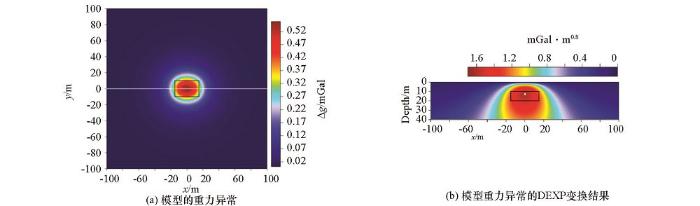
图1
直立棱柱体模型的重力异常(a)及其DEXP变换结果(b)
Fig.1
Gravity anomaly (a) of the rectangular prism model and its DEXP transform results (b)
图2
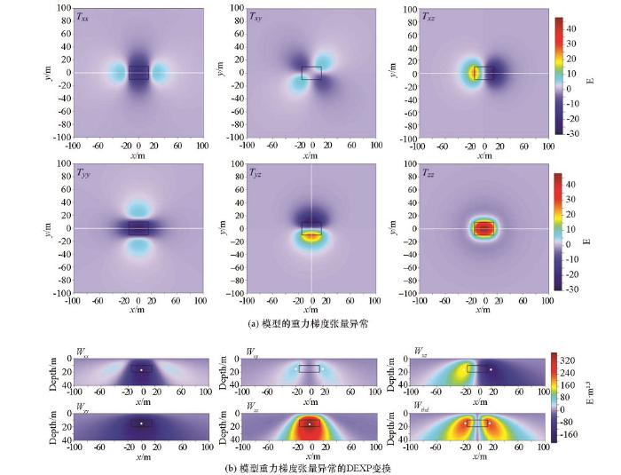
图2
直立棱柱体模型的重力梯度张量异常(a)及其DEXP变换结果(b)
Fig.2
Gravity gradient tensor components of the rectangular prism model (a) and its DEXP transform results (b)
在一定精度的数据基础及相同的数据处理方法上,如何减小其他影响因素对极值点深度成像结果的影响尤为重要。为了简化分析,笔者以重力垂向梯度的DEXP成像结果为例,分析数据的误差(噪声影响)、点距、计算范围和背景场对DEXP成像结果的影响。
2.1 DEXP变换的抗噪能力分析
图3
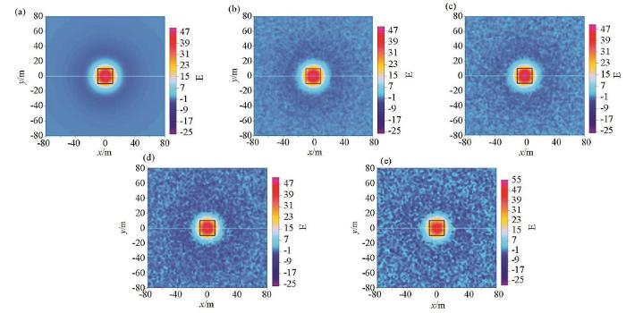
图3
加入不同高斯噪声的Tzz分量异常
Fig.3
Tzz component anomaly of the rectangular prism model with different Gauss noise
(a) Tzz component with 0% Gauss noise; (b) Tzz component with 1% Gauss noise; (c) Tzz component with 2% Gauss noise;(d) Tzz component with 5% Gauss noise; (e) Tzz component with 10% Gauss noise
图4
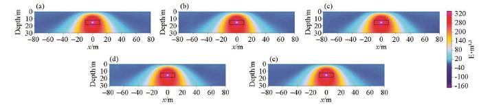
图4
与
Fig.4
DEXP transform results of Tzz component corresponding to
由图4加入了不同噪声的Tzz分量DEXP变换成像结果可知,其深度估计结果均与理论Tzz异常DEXP变换结果一致。这说明DEXP变换对噪声具有一定的压制作用,对加入较高比例的高斯噪声,其DEXP变换结果仍较准确。这是由于该算法主要基于向上延拓,而向上延拓属于低通滤波,因此受数据噪声的干扰很小。
2.2 数据点距对DEXP变换成像的影响
为了研究数据点距对异常体DEXP变换成像的影响,分别设置了3组不同点距(1、2以及5 m)进行试验研究。令直立棱柱体模型长a、宽b与高c分别为30、20与10 m,其中心埋深为30 m,剩余密度Δρ为1 g/cm3,计算范围为-70~70 m,向上延拓步长为1 m,总延拓高度为70 m。根据DEXP变换理论,即可得模型Tzz分量的深度成像结果,如图5所示。
图5
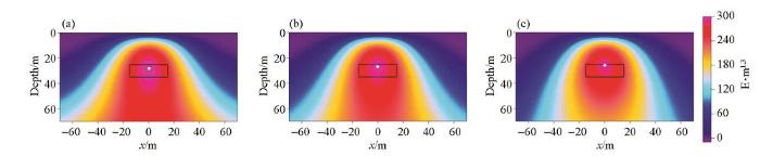
图5
数据点距为1 m(a)、2 m(b)和5 m(c)情况下的Tzz分量DEXP变换成像结果
Fig.5
DEXP transform results of Tzz component with data spaces of 1 m (a), 2 m (b) and 5 m (c)
由成像结果可知,当计算范围保持不变时,点距越小,所估计的模型埋深与理论中心埋深之间的差异越小。随着点距越大,所估计的深度结果更加偏离模型的中心深度位置,而往模型的上边界方向移动,并且其成像的整体形态越往异常体中心靠拢。
2.3 数据范围对DEXP变换成像的影响
图6
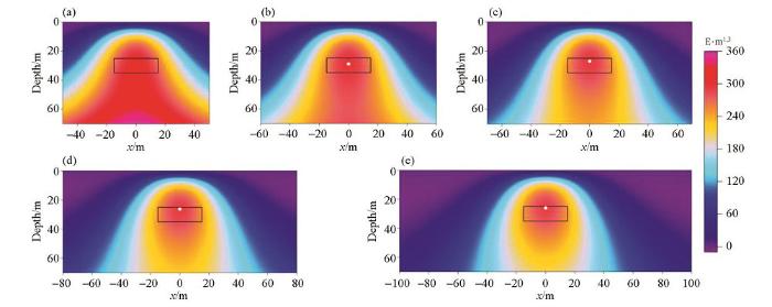
图6
计算范围为-50~50 m(a)、-60~60 m(b)、-70~70 m(c)、-80~80 m(d)、-100~100 m(e)时Tzz分量DEXP变换结果
Fig.6
DEXP transform results of Tzz component with data spatial ranges of -50~50 m (a), -60~60 m (b),-70~70 m (c), -80~80 m (d) and -100~100 m (e)
由成像结果可知:当点距保持不变时,若计算范围小于一定范围,由于变换过程中没有足够的场源信息,其成像形态过于向两侧分散,导致模型的DEXP变换成像结果在计算范围内不存在极值点;随着计算范围的增大,模型的DEXP变换结果异常形态开始向中心收敛,其极值点开始向模型中心位置移动,当到某个计算范围时,其极值点与模型中心位置重合,即DEXP变化所估计的深度与理论埋深一致、误差为零;若继续增大计算范围, DEXP变换结果对应极值点则会向场源的上边界移动,当增大到某一个计算范围之后,极值点位置不再发生移动,其位置收敛在场源的上边界附近。
2.4 背景场对DEXP变换结果的影响
图7
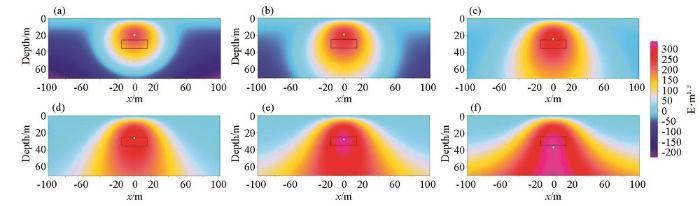
图7
加入-1E(a)、-0.5E(b)、-0.2E(c)、0E(d)、0.2E(e)和0.5E(f)的背景场之后的Tzz分量DEXP变换结果
Fig.7
DEXP transform results of Tzz component with background fields of -1E(a)、-0.5E(b)、-0.2E(c)、0E(d)、0.2E(e) 和 0.5E(f)
3 基于实际数据的影响因素分析
研究区位于路易斯安那州西南部,靠近德克萨斯州边界的Vinton盐丘区。区内为沉积岩相,地下发育盐丘构造。Vinton盐丘区全张量重力梯度(FTG)数据由Bell Geospace公司测得,采用南北向飞行测线,间隔为150 m,平均海拔75 m。测区范围为北纬30.07°~30.23°、西经93.53°~93.66°,总测线长度为1 087.5 km,测区面积为192.6 km2。图8a即为Vinton盐丘地区的重力异常数据。在进行DEXP变换时,Wp中的深度加权函数
图8
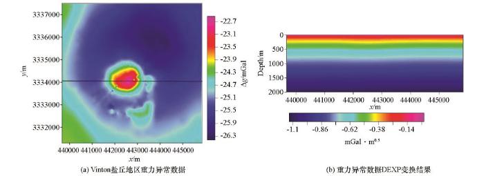
图8
Vinton盐丘地区重力异常(a)及其DEXP变换结果(b)
Fig.8
Gravity anomaly (a) in Vinton Salt Dome region and its DEXP transform results (b)
图9
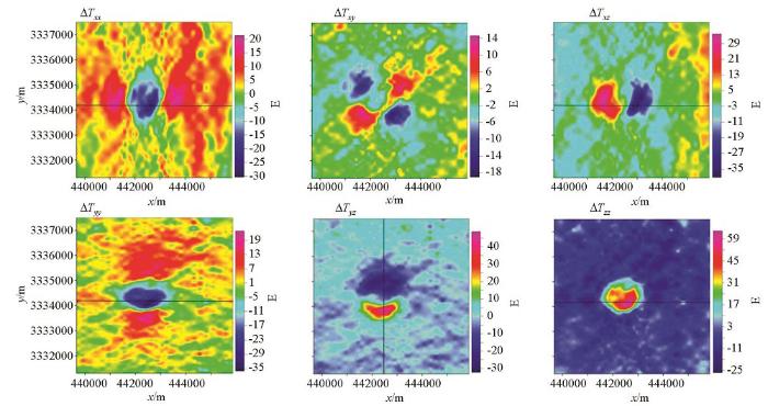
图9
Vinton盐丘地区的全张量重力梯度异常数据
Fig.9
The full gravity gradient tensor fields in Vinton Salt Dome region
图10
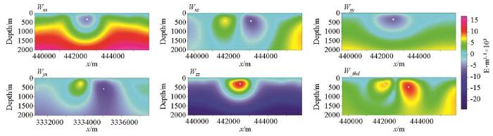
图10
Vinton盐丘地区全张量重力梯度数据的DEXP变换结果
Fig.10
DEXP transform results of the full gravity gradient tensor field data in Vinton Salt Dome region
图11
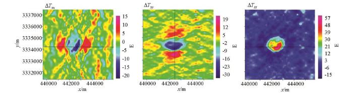
图11
Vinton盐丘地区ΔTxx、ΔTyy和ΔTzz分量分场之后的局部场
Fig.11
The residual fields of ΔTxx, ΔTyy and ΔTzz components after anomaly separation in Vinton Salt Dome region
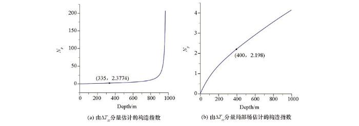
图12
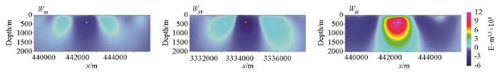
图12
Vinton盐丘地区ΔTxx、ΔTyy和ΔTzz分量的局部场DEXP变换成像结果
Fig.12
DEXP transform results of the residual fields of ΔTxx, ΔTyy and ΔTzz components after anomaly separation in Vinton Salt Dome region
图13
4 结论
笔者基于DEXP变换理论,将其应用于重力异常以及重力梯度张量极值点深度成像中,结果表明重力梯度张量的成像结果较好,并且重力梯度张量极值点深度成像不仅能够反映地下异常体的中心埋深,也能大致描述其边界位置。
同时也设置了多组直立棱柱体模型进行试验研究,以讨论不同因素(数据误差、点距、计算范围和背景场)对极值点深度成像结果的影响。结果表明:极值点深度成像法具有较好的抗噪能力,具有计算稳定性和准确性特点;当计算范围保持不变时,点距越小,所估计的模型埋深与理论中心埋深之间的差异越小;当点距保持不变时,计算范围由小变大,从不存在极值点到极值点开始向模型上边界方向移动直至模型上边界附近的某一深度值后不再变化;背景场对DEXP变换结果具有较大的影响,当其绝对值过大时,DEXP变换成像形态会发生很大的改变,甚至可能导致变换结果没有极值点。因此,在实际数据资料处理时,应该综合考虑相关因素对DEXP变换结果的影响,并且进行相关预处理(尤其是合适的局部异常提取)以提高深度估计结果的精度。
将DEXP变换应用于Vinton盐丘地区的全张量重力梯度数据成像中,首先对ΔTxx、ΔTyy和ΔTzz分量进行了分场处理,再将分场得到的局部场进行DEXP变换成像,得到了盐丘较为精确的中心埋深与构造指数。鉴于DEXP成像方法具有抗噪性、准确性以及便捷性,而且可以同时得到场源埋深与构造指数,也可以将其成像结果作为自约束信息引入三维物性反演之中,因而具有较好的应用前景,值得推广。
致谢
感谢Bell Geospace公司提供的全张量重力梯度数据!
参考文献
3-D inversion of gravity data
[J].DOI:10.1190/1.1444302 URL [本文引用: 1]
3-D inversion of gravity and magnetic data with depth resolution
[J].DOI:10.1190/1.1444550 URL [本文引用: 1]
Three-dimensional regularized focusing inversion of gravity gradient tensor component data
[J].DOI:10.1190/1.1778236 URL [本文引用: 1]
Understanding imaging methods for potential field data
[J].
DOI:10.1190/GEO2011-0078.1
URL
[本文引用: 1]

Several noniterative, imaging methods for potential field data have been proposed that provide an estimate of the 3D magnetization/density distribution within the subsurface or that produce images of quantities related or proportional to such distributions. They have been derived in various ways, using generalized linear inversion, Wiener filtering, wavelet and depth from extreme points (DEXP) transformations, crosscorrelation, and migration. We demonstrated that the resulting images from each of these approaches are equivalent to an upward continuation of the data, weighted by a (possibly) depth-dependent function. Source distributions or related quantities imaged by all of these methods are smeared, diffuse versions of the true distributions; but owing to the stability of upward continuation, resolution may be substantially increased by coupling derivative and upward continuation operators. These imaging techniques appeared most effective in the case of isolated, compact, and depth-limited sources. Because all the approaches were noniterative, computationally fast, and in some cases, produced a fit to the data, they did provide a quick, but approximate picture of physical property distributions. We have found that inherent or explicit depth-weighting is necessary to image sources at their correct depths, and that the best scaling law or weighting function has to be physically based, for instance, using the theory of homogeneous fields. A major advantage of these techniques was their speed, efficiently providing a basis for further detailed, follow-up modelling.
Application of the generalized linear inverse to the inversion of static potential data
[J].DOI:10.1190/1.1440686 URL [本文引用: 1]
Identification of sources of potential fields with the continuous wavelet transform: basic theory
[J].
Localization of maximum-depth gravity anomaly sources by a distribution of equivalent point masses
[J].DOI:10.1190/1.1487088 URL [本文引用: 1]
Potential field migration for rapid imaging of gravity gradiometry data
[J].
DOI:10.1111/j.1365-2478.2011.01005.x
URL
[本文引用: 1]
The geological interpretation of gravity gradiometry data is a very challenging problem. While maps of different gravity gradients may be correlated with geological structures present, maps alone cannot quantify 3D density distributions related to geological structures. 3D inversion represents the only practical tool for the quantitative interpretation of gravity gradiometry data. However, 3D inversion is a complicated and time-consuming procedure that is very dependent on the a priori model and constraints used. To overcome these difficulties for the initial stages of an interpretation workflow, we introduce the concept of potential field migration, and demonstrate how it can be applied for rapid 3D imaging of entire gravity gradiometry surveys. This method is based on a direct integral transformation of the observed gravity gradients into a subsurface density distribution that can be used for interpretation or as an a priori model for subsequent 3D regularized inversion. For large-scale surveys, we show how migration runs on the order of minutes compared to hours for 3D regularized inversion. Moreover, the results obtained from potential field migration are comparable to those obtained from regularized inversion with smooth stabilizers. We present a case study for the 3D imaging of FALCON airborne gravity gradiometry data from Broken Hill, Australia. We observe good agreement between results obtained from potential field migration and those generated by 3D regularized inversion.
DEXP: a fast method to determine the depth and the structural index of potential fields sources
[J].DOI:10.1190/1.2399452 URL [本文引用: 7]
3-D correlation imaging for gravity and gravity gradiometry data
[J].
3D migration for rapid imaging of total-magnetic-intensity data
[J].
DOI:10.1190/GEO2011-0425.1
URL
[本文引用: 1]
Three-dimensional potential field migration for rapid imaging of entire total-magnetic-intensity (TMI) surveys is introduced, and real time applications are discussed. Potential field migration is based on a direct integral transformation of the measured TMI data into a 3D susceptibility model, which could be directly used for interpretation or as an a priori model for subsequent regularized inversion. The advantage of migration is that it does not require any a priori information about the type of the sources present, nor does it rely on regularization as per inversion. Migration is very stable with respect to noise in measured data because the transform is reduced to the downward continuation of a function that is analytical everywhere in the subsurface. The 3D migration of TMI data acquired over the Reid-Mahaffy test site in Ontario, Canada is used as a test study. Our results are shown to be consistent with those results obtained from 3D regularized inversion as well as the known geology of the area. Interestingly, the migration of raw TMI data produces results very similar to the inversion of diurnally corrected and microleveled TMI data, suggesting that migration could be applied directly to real-time imaging during the acquisition.
Depth from extreme points method for gravity gradient tensor data
[J].
A fast interpretation of self-potential data using the depth from extreme points method
[J].
DOI:10.1190/GEO2012-0074.1
URL
[本文引用: 1]
We used a fast method to interpret self-potential data: the depth from extreme points (DEXP) method. This is an imaging method transforming self-potential data, or their derivatives, into a quantity proportional to the source distribution. It is based on upward continuing of the field to a number of altitudes and then multiplying the continued data with a scaling law of those altitudes. The scaling law is in the form of a power law of the altitudes, with an exponent equal to half of the structural index, a source parameter related to the type of source. The method is autoconsistent because the structural index is basically determined by analyzing the scaling function, which is defined as the derivative of the logarithm of the self-potential (or of its pth derivative) with respect to the logarithm of the altitudes. So, the DEXP method does not need a priori information on the self-potential sources and yields effective information about their depth and shape/typology. Important features of the DEXP method are its high-resolution power and stability, resulting from the combined effect of a stable operator (upward continuation) and a high-order differentiation operator. We tested how to estimate the depth to the source in two ways: (1) at the positions of the extreme points in the DEXP transformed map and (2) at the intersection of the lines of the absolute values of the potential or of its derivative (geometrical method). The method was demonstrated using synthetic data of isolated sources and using a multisource model. The method is particularly suited to handle noisy data, because it is stable even using high-order derivatives of the self-potential. We discussed some real data sets: Malachite Mine, Colorado (USA), the Sariyer area (Turkey), and the Bender area (India). The estimated depths and structural indices agree well with the known information.
Improving the local wavenumber method by automatic DEXP transformation
[J].
DOI:10.1016/j.jappgeo.2014.10.004
URL
[本文引用: 2]
In this paper we present a new method for source parameter estimation, based on the local wavenumber function. We make use of the stable properties of the Depth from EXtreme Points (DEXP) method, in which the depth to the source is determined at the extreme points of the field scaled with a power-law of the altitude. Thus the method results particularly suited to deal with local wavenumber of high-order, as it is able to overcome its known instability caused by the use of high-order derivatives. The DEXP transformation enjoys a relevant feature when applied to the local wavenumber function: the scaling-law is in fact independent of the structural index. So, differently from the DEXP transformation applied directly to potential fields, the Local Wavenumber DEXP transformation is fully automatic and may be implemented as a very fast imaging method, mapping every kind of source at the correct depth. Also the simultaneous presence of sources with different homogeneity degree can be easily and correctly treated. The method was applied to synthetic and real examples from Bulgaria and Italy and the results agree well with known information about the causative sources. (C) 2014 Elsevier B.V.
Determination of the maximum-depth to potential field sources by a maximum structural index method
[J].
DOI:10.1016/j.jappgeo.2012.10.009
URL
[本文引用: 1]
Thanks to the direct relationship between structural index and depth to sources we work out a simple and fast strategy to obtain the maximum depth by using the semi-automated methods, such as Euler deconvolution or depth-from-extreme-points method (DEXP).The proposed method consists in estimating the maximum depth as the one obtained for the highest allowable value of the structural index (N-max). N-max be easily determined, since it depends only on the dimensionality of the problem (2D/3D) and on the nature of the analyzed field (e.g., gravity field or magnetic field). We tested our approach on synthetic models against the results obtained by the classical Bott Smith formulas and the results are in fact very similar, confirming the validity of this method. However, while Bolt Smith formulas are restricted to the gravity field only, our method is applicable also to the magnetic field and to any derivative of the gravity and magnetic field. Our method yields a useful criterion to assess the source model based on the (partial derivative f/partial derivative x)(max)/f(max) ratio.The usefulness of the method in real cases is demonstrated for a salt wall in the Mississippi basin, where the estimation of the maximum depth agrees with the seismic information. (C) 2012 Elsevier B.V.]]>
EULDPH: A new technique for making computer assisted depth estimates from magnetic data
[J].DOI:10.1190/1.1441278 URL [本文引用: 1]
3D inversion of airborne gravity-gradiometry data using cokriging
[J].
DOI:10.1190/GEO2013-0393.1
URL
[本文引用: 1]
We developed a new method for interpretation of airborne gravity gradiometry data, based on cokriging inversion. The cokriging method that we evaluated minimized the theoretical estimation error variance by using auto- and crosscorrelations of several variables. It does not require iterations and can easily include complex a priori information. Moreover, the smoothing effects in the inverted density structure model can be reduced to a certain extent due to the anisotropy constrain in the covariance model. We compared the recovered models obtained by inverting the different combinations of gravity-gradient components to understand how different component combinations contributed to the resolution of the recovered model. The results indicated that including multiple components for inversion increased the resolution of the recovered density model and improved the structure delineation. Moreover, in the case in which the parameters of the variogram model are not well chosen, cokriging with multicomponent combinations can still correctly recover the geometry of the targeted sources. The survey data of the Vinton dome were considered as a case study. The results of the inversion were in good agreement with the known formation in the region. This supports the validity of our method.
全张量重力梯度数据的综合分析与处理解释
[D].
Comprehensive analysis, processing and interpretation of the full tensor gravity gradient data
[D].
利用比值DEXP进行重力梯度数据深度成像
[J].针对传统 DEXP 快速成像结果依赖于地质体构造指数的缺点,笔者提出了利用重力异常不同阶垂向导数比值 DEXP 的方法。该方法使得成像结果独立于地质体构造指数。地质体的深度估计完全自动化,仅需要寻找比值 DEXP 成像结果的极大值点位置。通过该方法估计出的深度结果,可以进行地质体构造指数的估计。通过模型试验,证明该方法能准确地估计出地质体的深度位置以及地质体的类型。将该方法应用到 Bell Geospace 公司在 Vinton Dome 测得的 Air- -FTG 全张量重力梯度数据中取得了很好的结果。
Using ratio DEXP for depth imaging of gravity gradient data
[J].
Vinton salt dome, CalcasieuParish, Louisiana
[J].
Interpretation of tensor gravity data using an adaptive tilt angle method
[J].
DOI:10.1111/1365-2478.12039
URL
[本文引用: 1]
Full Tensor Gravity Gradiometry (FTG) data are routinely used in exploration programmes to evaluate and explore geological complexities hosting hydrocarbon and mineral resources. FTG data are typically used to map a host structure and locate target responses of interest using a myriad of imaging techniques. Identified anomalies of interest are then examined using 2D and 3D forward and inverse modelling methods for depth estimation. However, such methods tend to be time consuming and reliant on an independent constraint for clarification. This paper presents a semi-automatic method to interpret FTG data using an adaptive tilt angle approach. The present method uses only the three vertical tensor components of the FTG data (T-zx, T-zy and T-zz) with a scale value that is related to the nature of the source (point anomaly or linear anomaly). With this adaptation, it is possible to estimate the location and depth of simple buried gravity sources such as point masses, line masses and vertical and horizontal thin sheets, provided that these sources exist in isolation and that the FTG data have been sufficiently filtered to minimize the influence of noise. Computation times are fast, producing plausible results of single solution depth estimates that relate directly to anomalies. For thick sheets, the method can resolve the thickness of these layers assuming the depth to the top is known from drilling or other independent geophysical data. We demonstrate the practical utility of the method using examples of FTG data acquired over the Vinton Salt Dome, Louisiana, USA and basalt flows in the Faeroe-Shetland Basin, UK. A major benefit of the method is the ability to quickly construct depth maps. Such results are used to produce best estimate initial depth to source maps that can act as initial models for any detailed quantitative modelling exercises using 2D/3D forward/inverse modelling techniques.
3-D radial gravity gradient inversion
[J].
DOI:10.1093/gji/ggt307
URL
[本文引用: 1]
We have presented a joint inversion of all gravity-gradient tensor components to estimate the shape of an isolated 3-D geological body located in subsurface. The method assumes the knowledge about the depth to the top and density contrast of the source. The geological body is approximated by an interpretation model formed by an ensemble of vertically juxtaposed 3-D right prisms, each one with known thickness and density contrast. All prisms forming the interpretation model have a polygonal horizontal cross-section that approximates a depth slice of the body. Each polygon defining a horizontal cross-section has the same fixed number of vertices, which are equally spaced from 0 degrees to 360 degrees and have their horizontal locations described in polar coordinates referred to an arbitrary origin inside the polygon. Although the number of vertices forming each polygon is known, the horizontal coordinates of these vertices are unknown. To retrieve a set of juxtaposed depth slices of the body, and consequently, its shape, our method estimates the radii of all vertices and the horizontal Cartesian coordinates of all arbitrary origins defining the geometry of all polygons describing the horizontal cross-sections of the prisms forming the interpretation model. To obtain a stable estimate that fits the observed data, we impose constraints on the shape of the estimated body. These constraints are imposed through the well-known zeroth- and first-order Tikhonov regularizations allowing, for example, the estimate of vertical or dipping bodies. If the data do not have enough in-depth resolution, the proposed inverse method can obtain a set of stable estimates fitting the observed data with different maximum depths. To analyse the data resolution and deal with this possible ambiguity, we plot the l(2)-norm of the residuals (s) against the estimated volume (v(p)) produced by a set of estimated sources having different maximum depths. If this s x v(p) curve (s as a function of v(p)) shows a well-defined minimum of s, the data have enough resolution to recover the shape of the body entirely. Conversely, if the observed data do not have enough resolution, some estimates with different maximum depths produce practically the same minimum value of s on the s x v(p) curve. In this case, the best estimate among a suite of estimates producing equally data fits is the one fitting the gravity-gradient data and producing the minima of both the source's bottom depth and volume. The histograms of the residuals can be used to quantify and remove systematic errors in the data. After removing these errors, we confirmed the ability of our method to recover the source geometry entirely (or its upper part only), if the data have sufficient (or insufficient) in-depth resolution. By inverting the gravity-gradient data from a survey over the Vinton salt dome (Louisiana, USA) with a density contrast of 0.55 g cm(-3), we estimated a massive cap rock whose maximum depth attains 460 +/- 10 m and its shallowest portion is elongated in the northeast-southwest direction.
重力全张量数据联合欧拉反褶积法研究及应用
[J].
The study on the joint Euler deconvolution method of full tensor gravity data
[J].
Vinton dome地区全张量重力异常的解释
[J].
The interpretation of full tensor gravity gradient data in Vinton dome area
[J].
重力梯度张量数据的三维反演方法与应用
[J].全张量重力梯度测量技术日趋成熟,已成为地球物理勘探的重要方法之一。本文将重力异常三维反演技术应用于重力梯度张量数据反演,并针对重力梯度张量数据,构建了联合反演目标函数,同时引入投影梯度算法对反演求解过程施加约束。通过理论模型试验和实际资料的应用,表明了方法的可行性和应用前景。
3-D inversion method and application of gravity gradient tensor data
[J].
