Research on fast three-dimensional forward algorithm of magnetotelluric sounding based on vector finite element
GU Guan-Wen1,2(), WU Ye1,2, SHI Yan-Bin1,2
1. School of Earth Sciences, Institute of Disaster Prevention, Langfang 065201, China 2. Hebei Key Laboratory of Earthquake Dynamics, Langfang 065201, China
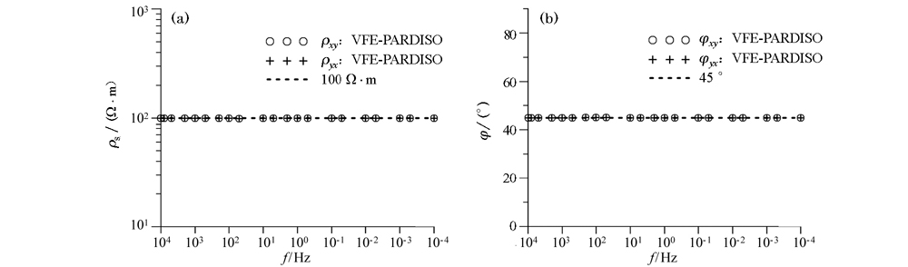
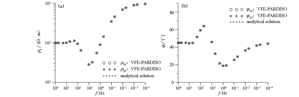
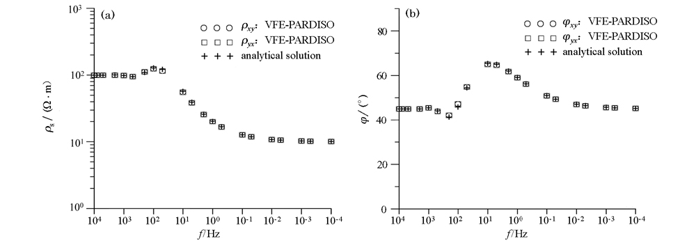
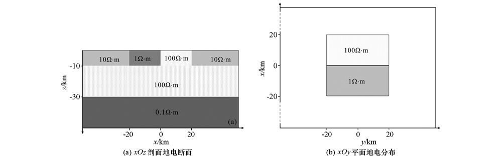
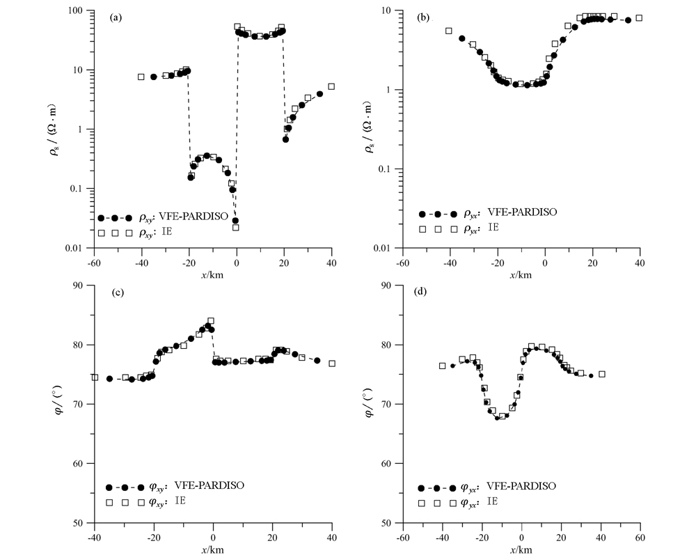
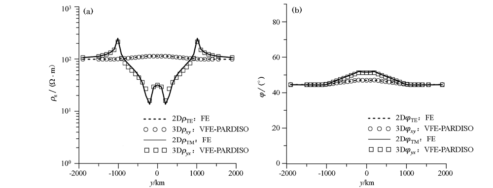
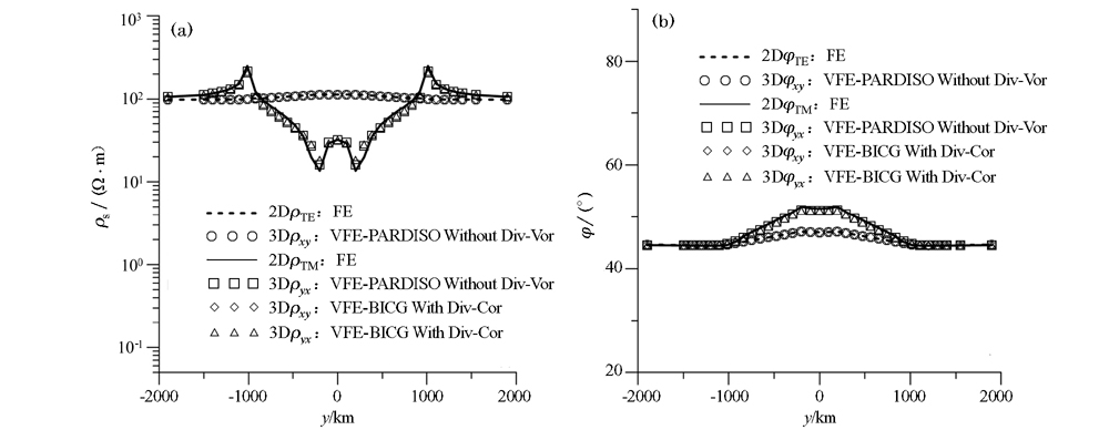
The finite element method has the characteristics of strong adaptability in simulating the electromagnetic response of rugged topography and complex geological bodies. In recent years, it has been widely used in the three-dimensional (3D) forward modeling of magnetotelluric (MT) sounding. However, the finite element method also has some shortcomings in terms of computational efficiency. The large amount of calculation and long running time of the method are the main factors that lead to the lag of the practical process of the 3D MT inversion technology based on the finite element method compared with the 3D MT inversion technology based on the finite difference method. In order to improve the 3D forward speed of MT, the authors adopt the forward modeling scheme which uses the direct solver PARDISO and does not need divergence correction to solve the large-scale linear equations corresponding to the vector finite element method, and obtain the MT response of the geoelectric model under such different terrain conditions as flat and rugged topography. Under the conditions of medium-scale calculation, through the comparison between the direct solution method without divergence correction and the iterative solution method with divergence correction, the authors have detected that the direct solution method without divergence correction has advantages in calculation accuracy and calculation time, especially in the calculation. In terms of time, the ratio of the calculation speed of the direct solution and the iterative solution is raised by more than ten times.
顾观文, 武晔, 石砚斌. 基于矢量有限元的大地电磁快速三维正演研究[J]. 物探与化探, 2020, 44(6): 1387-1398.
GU Guan-Wen, WU Ye, SHI Yan-Bin. Research on fast three-dimensional forward algorithm of magnetotelluric sounding based on vector finite element. Geophysical and Geochemical Exploration, 2020, 44(6): 1387-1398.
Xu K J, Li T L, Zhang H, et al. Three-dimensional magnetotelluric forward modeling using integral equation[J]. Northwestern Seismological Journal, 2006(2):104-107.
Ren Z Y, Chen C J, Tang J T, et al. A new integral equation approach for 3D magnetotelluric modeling[J]. Chinese Journal of Geophysics, 2017,60(11):4506-4515.
[4]
Mackie R L, Madden T R, Wannamaker P. 3-D magnetotelluric modeling using difference equations-theory and comparisons to integral equation solutions[J]. Geophysics, 1993,58:215-226.
[5]
Mackie R L, Smith T J, Madden T R. 3-D electromagnetic modeling using difference equations:The Magnetotelluric Example[J]. Radio Sci., 1994,29:923-935.
[6]
Newman G A, Alumbaugh D L. Three-dimensional induction logging problems.Part I. An integral equation solution and model comparisons[J]. Geophysics, 2002,67:484-491.
[7]
谭捍东, 余钦范, John Booker, 等. 大地电磁三维交错网格有限差分正演[J]. 地球物理学报, 2003,46(5):705-711.
[7]
Tan H D, Yu Q F, Booker J, et al. Magnetotelluric three-dimension modeling using the staggered-grid finite difference method[J]. Chinese Journal of Geophysics, 2003,46(5):705-711.
Dong H, Wei W B, Ye G F, et al. Study of three-dimensional magnetotelluric inversion including surface topography based on Finite-difference method[J]. Chinese Journal of Geophysics, 2014,57(3):939-952.
[9]
Mitsuhata Y, Uchida T. 3D magnetotelluric modeling using the T-Ω finite-element method[J]. Geophysics, 2004,69(1):108-119.
Tang J T, Zhang L C, Gong J Z, et al. 3D frequency domain controlled source electromagnetic numericalmodeling with coupled finite-infinite element method[J]. Journal of Central South University:Science and Technology, 2014,45(4):1251-1260.
[11]
Shi X, Utada H, Wang J, et al. Three-dimensional magnetotelluric forward modelling using vector finite element method combined with divergence corrections(VFE++)[R]// 2004,17th IAGA WG1.2 Workshop on electromagnetic Induction in the Earth.Hyderabad.
[12]
Nam N J, Kim H J, Song Y, et al. 3D magnetotelluric modelling inluding surface topography[J]. Geophysical Prospecting, 2007,55(2):277-287.
[13]
Ren Z Y, Kaischeuer T, Greenhalgh S, et al. A goal-oriented adaptive finite-element approach for plane wave 3D electromagnetic modeling[J]. Geophys. J. Int., 2013,194:700-718.
Gu G W, Wu W L, Li T L. Modeling for the effect of magnetotelluric 3D topography based on the vector finite-element method[J]. Journal of Jilin University:Earth Science Edition, 2014,44(5):1678-1686.
Yin C C, Zhang B, Liu Y H, et al. A goal-oriented adaptive algorithm for 3D magnetotelluric forward modeling[J]. Chinese Journal of Geophysics, 2017,60(1):327-336.
Wang G, Wei W B, Jin S, et al. A study on the electrical structure of eastern Gangdese metallogenic belt[J]. Chinese Journal of Geophysics, 2017,60(8):2993-3003.
Yu H, Deng J Z, Chen H, et al. Three-dimensional magnetotelluric inversion under topographic relief based on the limited-memory quasi-Newton algorithm(L-BFGS)[J]. Chinese Journal of Geophysics, 2019,62(8):3175-3188.
Cui T F, Chen X B, Zhan Y, et al. Characteristics of deep electrical structure and seismogenic structure beneath Anhui Huoshan earthquake area[J]. Chinese Journal of Geophysics, 2020,63(1):256-269.
Yang W C, Jin S, Zhang L L, et al. The three-dimensional resistivity structures of the lithosphere beneath the Qinghai-Tibet Plateau[J]. Chinese Journal of Geophysics, 2020,63(3):817-827.
Tang J T, Ren Z Y, Hua X R. The forward modeling and inversion ingeophysical electromagnetic field[J]. Progress in Geophysics, 2007,22(4):1181-1194.
[21]
Smith J T. Conservative modeling of 3D electromagnetic fields, Part I, Properties and error analysis[J]. Geophysics, 1996,61:1308-1318.
doi: 10.1190/1.1444054
[22]
Farquharson C G, Miensopust M P. Three-dimensional finite-element modeling of magnetotelluric data with a divergence correction[J]. Journal of Applied Geophysics, 2011,75(4):699-710.
doi: 10.1016/j.jappgeo.2011.09.025
[23]
Schenk O, Gärtner K. Solving unsymmetric sparse systems of linear equations with PARDISO[J]. Future Generation Computer Systems, 2004,20:475-487.
doi: 10.1016/j.future.2003.07.011
[24]
AmestoyP R, Duff I S, L’Excellent J Y, et al. A fully asynchronous multifrontal solver using distributed dynamic scheduling[J]. SIAM J. Matrix Anal. Appl., 2002,23(1):15-41.
doi: 10.1137/S0895479899358194
[25]
Amestoy P R, Guermouche A, L’Excellent J Y, et al. Hybrid schedulingfor the parallel solution of linear systems[J]. Parallel Computing, 2006,32(2):136-156.
doi: 10.1016/j.parco.2005.07.004
[26]
Streich R. 3D finite-difference frequency-domain modeling of controlled-source electromagnetic data: Direct solution and optimization for high accuracy[J]. Geophysics, 2009,74(5):F95-F105.
doi: 10.1190/1.3196241
[27]
Puzyrev V, Koldan J, De La Puente J, et al. A parallel finite-element method for three-dimensional controlled-source electromagnetic forward modeling[J]. Geophysical Journal International, 2013,193(2):678-693.
doi: 10.1093/gji/ggt027
[28]
Kordy M, Wannamaker K, Maris V, et al. 3D magnetotelluric inversion including topography using deformed hexahedral edge finite elements and direct solvers parallelized on SMP computers—Part I: forward problem and parameter Jacobians[J]. Geophys. J. Int., 2016,204:74-93.
doi: 10.1093/gji/ggv410
Tang J T, Ren Z Y, Zhou C, et al. Frequency-domain electromagnetic methods for exploration of the shallow subsurface: A review[J]. Chinese Journal of Geophysics, 2015,58(8):2681-2705.
[30]
Siripunvaraporn W, Egbert G, Lenbury Y. Numerical accuracy of magnetotelluric modeling: A comparison of finite difference approximations[J]. Earth Planets Space, 2002,54:721-725.
doi: 10.1186/BF03351724
[31]
徐世浙. 地球物理中的有限单元法[M]. 北京: 科学出版社, 1994.
[31]
Xu S Z. Finite element method in Geophysics[M]. Beijing: Science Press, 1994.
[32]
金建铭. 电磁场有限元方法[M]. 西安: 西安电子科技大学出版社, 1998: 176-189.
[32]
Jin J M. The Finite element method in electromagnecic fields [M]. Xi’an: Xidian University Press, 1998: 176-189.
[33]
Gould N I M, Scott J A, H Y F. A numerical evaluation of sparse direct solvers for the solution of large sparse symmetric linear systems of equations[J]. ACM Transactions on Mathematical Software, 2007,33(2):300-325.
[34]
Newman G A, Alumbaugh D L. Three-dimensional magnetotelluric inversion using non-linear conjugate gradients[J]. Geophys. J. Int., 2000,140:410-424.
doi: 10.1046/j.1365-246x.2000.00007.x
Tan H D, Wei W B, Deng M, et al. General use formula in MT tensor impedance[J]. Oil Geophysical Prospecting, 2004,39(1):113-116.
[36]
Zhdanov M S, Varentov I M, Weaver J T, et al. Methods for modeling electromagnetic fields: Results from COMMEMI——The international project on the comparison of modeling methods for electromagnetic induction[J]. Journal of Applied Geophysics, 1997,37:133-271.
doi: 10.1016/S0926-9851(97)00013-X
[37]
Wannamaker P E, Stodt J A, Rijo L. Two-dimensional topographic responses in magnetotelluric model using finite elements[J]. Geophysics, 1986,51(11):2121-2144.
Qin C, Wang X B, Zhao N. Parallel three-dimensional forward modeling and inversion of magnetotelluric based on a secondary field approach[J]. Chinese Journal of Geophysics, 2017,60(6):2456-2468.
[39]
Chen P F, Hou Z H, Fan G H. Three-dimension topographic responses in MT using finite difference method[J]. Acta Seismologica Sinica, 1998,11(5):631-635.
doi: 10.1007/s11589-998-0079-6